Linearized steam turbine flow characteristic. Part 2. Example of construction for the PT-80 turbine in MATLAB
Preface to the first part
Steam turbine modeling is the daily task of hundreds of people in our country. Instead of the word model, it is customary to say the expenditure characteristic . The consumption characteristics of steam turbines are used in solving such tasks as calculating the specific consumption of equivalent fuel for electricity and heat produced by CHP; optimization of CHP operation; planning and maintenance of CHP modes.
I have developed a new steam turbine flow characteristic - a linearized steam turbine flow characteristic. The developed expense characteristic is convenient and effective in the solution of the specified tasks. However, at the moment it is described in only two scientific papers:
- Optimization of CHP operation in the conditions of the wholesale electricity and capacity market in Russia ;
- Computational methods for determining the specific consumption of reference fuel CHP for the released electric and thermal energy in the mode of combined development .
And now in my blog I would like to:
- firstly, to answer basic questions about new consumption characteristics in simple and accessible language (see Linearized characteristics of a steam turbine. Part 1. Main questions );
- secondly, to provide an example of constructing a new expenditure characteristic, which will help to understand both the construction method and the properties of the characteristic (see below);
- thirdly, to refute two well-known statements regarding the operating modes of the steam turbine (see Linearized steam turbine flow characteristic. Part 3. We will dispel the myths about the operation of the steam turbine ).
1. Baseline
Baseline data for the construction of linearized flow characteristics can be
- the actual values of power Q 0 , N, Q p , Q t measured in the operation of the steam turbine,
- nomograms q t gross from normative technical documentation.
Of course, the actual instantaneous values of Q 0 , N, Q n , Q t are ideal source data. Collecting such data is time consuming.
In cases where the actual values of Q 0 , N, Q n , Q t are not available, it is possible to process nomograms q t gross. They, in turn, were obtained on the basis of measurements. For more information about turbine testing, see V. Gornstein. and others. Methods of optimization of power systems .
2. Algorithm for constructing linearized consumption characteristics
The construction algorithm consists of three steps.
- Converting nomograms or measurement results to a table view.
- Linearization of steam turbine flow characteristics.
- Determining the boundaries of the adjustment range of the steam turbine.
When working with nomograms q t gross, the first step is carried out quickly. This work is called digitizing . Digitizing 9 nomograms for the current example took me about 40 minutes.
The second and third steps require the use of math packages. I love and use MATLAB for many years. My example of building a linearized flow characteristic is made exactly in it. An example can be downloaded from the link , run and independently figure out the method for constructing linearized consumption characteristics.
The flow characteristic for the considered turbine was built for the following fixed values of the mode parameters:
- single stage operation
- medium pressure steam pressure = 13 kgf / cm2,
- low pressure steam pressure = 1 kgf / cm2.
The content of the archive Chuchueva-PT-80-linear-characteristic-curve.rar .
1) Nomograms of specific consumption q t gross for electricity generation (the marked red points are digitized - transferred to the table):
- PT80_qt_Qm_eq_0_digit.png,
- PT80_qt_Qm_eq_100_digit.png,
- PT80_qt_Qm_eq_120_digit.png,
- PT80_qt_Qm_eq_140_digit.png,
- PT80_qt_Qm_eq_150_digit.png,
- PT80_qt_Qm_eq_20_digit.png,
- PT80_qt_Qm_eq_40_digit.png,
- PT80_qt_Qm_eq_60_digit.png,
- PT80_qt_Qm_eq_80_digit.png.
2) Result of digitization (each psv file corresponds to a png file):
- PT-80_Qm_eq_0.csv,
- PT-80_Qm_eq_100.csv,
- PT-80_Qm_eq_120.csv,
- PT-80_Qm_eq_140.csv,
- PT-80_Qm_eq_150.csv,
- PT-80_Qm_eq_20.csv,
- PT-80_Qm_eq_40.csv,
- PT-80_Qm_eq_60.csv,
- PT-80_Qm_eq_80.csv.
3) MATLAB script with calculations and graphing:
- PT_80_linear_characteristic_curve.m
4) The result of the digitization of nomograms and the result of the construction of linearized consumption characteristics in tabular form:
- PT_80_linear_characteristic_curve.xlsx.
Step 1. Converting nomograms or measurement results to a table
1. Processing of raw data
The initial data for our example are nomograms q t gross.
To convert the set of nomograms into digital form, a special tool is needed. I reused a web application for this purpose. The application is simple, convenient, but does not have enough flexibility to automate the process. Some work has to be done manually.
At this step, it is important to digitize the extreme points of nomograms that define the boundaries of the adjustment range of the steam turbine .
The job was to mark the points of expenditure characteristics in each png file using the application , download the resulting csv and collect all the data in one table. The result of digitization can be found in the file PT-80-linear-characteristic-curve.xlsx, sheet "PT-80", the table "Initial data".
2. Reduction of units of measure to units of power
Next on the sheet "PT-80" we calculate the values of Q 0 by the formula
$$ display $$ \ begin {equation} Q_0 = \ frac {q_T \ cdot N} {1000} + Q_P + Q_T \ qquad (1) \ end {equation} $$ display $$
and we give all the initial values to MW. Calculations are implemented using MS Excel.
The resulting table “Initial data (power units)” is the result of the first step of the algorithm.
Step 2. Linearization of steam turbine flow characteristics
1. Check MATLAB operation
At this step, you need to install and open MATLAB version not lower than 7.3 (this is the old version, the current 8.0). In MATLAB, open the PT_80_linear_characteristic_curve.m file, run it and verify that it works. Everything works correctly if you saw the following message on the command line following the script startup:
PT_80_linear_characteristic_curve.xlsx 1 : a(N) = 2.317, a(Q) = 0.621, a(Q) = 0.255, a0 = 33.874 = 0.006, (0.57%) = 37 If you have any errors, then figure it out yourself how to fix them.
2. Calculations
All calculations are implemented in the file PT_80_linear_characteristic_curse.m. Consider it in parts.
1) Specify the name of the source file, the sheet, the range of cells containing the table “Source data (power units)” obtained in the previous step.
XLSFileName = 'PT_80_linear_characteristic_curve.xlsx'; XLSSheetName = 'PT-80'; XLSRange = 'F3:I334'; 2) We consider the original data in MATLAB.
sourceData = xlsread(XLSFileName, XLSSheetName, XLSRange); N = sourceData(:,1); Qm = sourceData(:,2); Ql = sourceData(:,3); Q0 = sourceData(:,4); fprintf(' %s %1.0f \n', XLSFileName, toc); We use the variable Qm for the vapor flow of the average pressure Qn, the index m from the middle is the average; similarly, we use the variable Ql for the low-pressure steam flow rate Q n , the l index from low is low.
3) Define the coefficients α i .
Recall the general formula of consumption characteristics
$$ display $$ \ begin {equation} Q_0 = f (N, Q_P, Q_T) \ qquad (2) \ end {equation} $$ display $$
and specify the independent (x_digit) and dependent (y_digit) variables.
x_digit = [N Qm Ql ones(size(N,1),1)]; % N, Q, Q, y_digit = Q0; % Q0 If you don’t understand why there is a unit vector in the x_digit matrix (the last column), then read the materials on linear regression. On the topic of regression analysis, I recommend the book by Draper N., Smith H. Applied regression analysis . New York: Wiley, In press, 1981. 693 p. (available in Russian).
Equation of linearized flow characteristics of a steam turbine
$$ display $$ \ begin {equation} Q_0 = \ alpha_N \ cdot N + \ alpha_P \ cdot Q_P + \ alpha_T \ cdot Q_T + \ alpha_0 \ qquad (3) \ end {equation} $$ display $$
is a multiple linear regression model. The coefficients α i will be determined using the "great good of civilization" - the method of least squares. Separately, I note that the least squares method was developed by Gauss in 1795.
In MATLAB this is done in one line.
A = regress(y_digit, x_digit); fprintf(': a(N) = %4.3f, a(Q) = %4.3f, a(Q) = %4.3f, a0 = %4.3f\n',... A); Variable A contains the required coefficients (see the message in the MATLAB command line).
Thus, the obtained linearized flow characteristic of the steam turbine PT-80 has the form
$$ display $$ \ begin {equation} Q_0 = 2.317 \ cdot N + 0.621 \ cdot Q_P + 0.255 \ cdot Q_T + 33.874 \ qquad (4) \ end {equation} $$ display $$
4) We estimate the linearization error of the obtained flow characteristic.
y_model = x_digit * A; err = abs(y_model - y_digit) ./ y_digit; fprintf(' = %1.3f, (%4.2f%%)\n\n', mean(err), mean(err)*100); The linearization error is 0.57% (see the message on the MATLAB command line).
To assess the convenience of using the linearized flow characteristics of a steam turbine, we will solve the problem of calculating the high-pressure steam flow Q 0 with known values of the load N, Q n , Q t .
Let N = 82.3 MW, Q n = 55.5 MW, Q t = 62.4 MW, then
$$ display $$ \ begin {equation} Q_0 = 2.317 \ cdot 82.3 + 0.621 \ cdot 55.5 + 0.255 \ cdot 62.4 + 33.874 = 274.9 \ qquad (5) \ end {equation} $$ display $$
Let me remind you that the average calculation error is 0.57%.
Let us return to the question, what is the linearized flow characteristic of a steam turbine more fundamentally more convenient than nomograms of specific consumption qt gross for power generation? To understand the fundamental difference in practice, solve two problems.
- Calculate the value of Q 0 with the specified accuracy using nomograms and your eyes.
- Automate the process of calculating Q 0 using nomograms.
Obviously, in the first task, determining the values of q t gross by eye is fraught with gross errors.
The second task is cumbersome for automation. Since the q t gross values are nonlinear , for such automation the number of digitized points is ten times more than in the current example. Digitization alone is not enough; it is also necessary to implement an interpolation algorithm (finding values between points) of nonlinear gross values.
Step 3. Determining the limits of the adjustment range of the steam turbine
1. Calculations
To calculate the adjustment range, we use another “blessing of civilization” - the convex hull method, convex hull.
In MATLAB, this is done as follows.
indexCH = convhull(N, Qm, Ql, 'simplify', true); index = unique(indexCH); regRange = [N(index) Qm(index) Ql(index)]; regRangeQ0 = [regRange ones(size(regRange,1),1)] * A; fprintf(' = %d\n\n', size(index,1)); The convhull () method determines the boundary points of the adjustment range specified by the values of the variables N, Qm, Ql. The indexCH variable contains vertices of triangles constructed using the Delaunay triangulation. The variable regRange contains the boundary points of the adjustment range; The regRangeQ0 variable is the high-pressure steam consumption for the boundary points of the adjustment range.
The result of the calculations can be found in the file PT_80_linear_characteristic_curve.xlsx, sheet “PT-80-result”, table “Limits of the adjustment range”.
Linearized flow characteristic built. It is a formula (4) and 37 points that define the boundaries (shell) of the adjustment range in the corresponding table.
2. Check
When automating the Q 0 calculation processes, it is necessary to check whether a certain point with N, Q n , Q t values is within the adjustment range or outside of it (the mode is not technically feasible). In MATLAB, you can do this as follows.
Set the values of N, Q n , Q t , which we want to check.
n = 75; qm = 120; ql = 50; We are checking.
in1 = inpolygon(n, qm, regRange(:,1),regRange(:,2)); in2 = inpolygon(qm, ql, regRange(:,2),regRange(:,3)); in = in1 && in2; if in fprintf(' N = %3.2f , Q = %3.2f , Q = %3.2f \n', n, qm, ql); else fprintf(' N = %3.2f , Q = %3.2f , Q = %3.2f ( )\n', n, qm, ql); end The check is carried out in two steps:
- in1 variable indicates whether the values of N, Q p fell inside the projection of the shell on the N, Q p axis;
- similarly, the variable in2 indicates whether the values of Qn, Qt fell inside the shell projection on the Qn, Qt axes.
If both variables are equal to 1 (true), then the desired point is inside the shell that specifies the adjustment range of the steam turbine.
Illustration of the resulting linearized steam turbine flow characteristic
We received the most “generous benefits of civilization” in terms of illustrating the results of calculations.
It must first be said that the space in which we build graphs, that is, the space with the axes x - N, y - Q m , z - Q 0 , w - Q n , is called the mode space (see Optimization of the CHP operation under conditions the wholesale market for electricity and power in Russia
). Each point of this space defines a certain mode of operation of the steam turbine. Mode may be- technically feasible, if the point is inside the shell that defines the adjustment range,
- not technically feasible if the point is outside this shell.
If we talk about the condensation mode of operation of the steam turbine (Qn = 0, Qt = 0), then the linearized flow characteristic is a straight line segment . If we talk about a T-type turbine, the linearized flow characteristic is a flat polygon in a three-dimensional mode space with the axes x - N, y - Q t , z - Q 0 , which is easy to visualize. For a PT-type turbine, visualization is the most difficult, since the linearized flow characteristic of such a turbine represents a flat polygon in four-dimensional space (for explanations and examples, see Optimization of CHP operation in the conditions of the wholesale electricity and power market of Russia, section Linearization of flow characteristics of the turbine ).
1. Illustration of the obtained linearized steam turbine flow characteristics
Construct the values of the table “Initial data (units of power)” in the mode space.
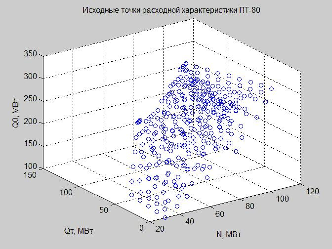
Fig. 3. Initial points of the discharge characteristics in the mode space with the axes x - N, y - Q t , z - Q 0
Since we cannot build dependencies in four-dimensional space, we have not yet reached such a good of civilization, we operate with the values of Qn as follows: eliminate them (Fig. 3), fix (Fig. 4) (see the charting code in MATLAB).
Fix the value of Q p = 40 MW and construct the source points and the linearized flow characteristic.
Fig. 4. Reference points of consumption characteristics (blue points), linearized consumption characteristics (green flat polygon)
Let us return to the formula of linearized expenditure characteristic (4) obtained by us. If we fix Q n = 40 MW MW, then the formula will look like
$$ display $$ \ begin {equation} Q_0 = 2.317 \ cdot N + 0.255 \ cdot Q_T + 58.714 \ qquad (6) \ end {equation} $$ display $$
This model defines a flat polygon in three-dimensional space with the axes x - N, y - Q t , z - Q 0 by analogy with a T-type turbine (we see it in Fig. 4).
Many years ago, when we developed nomograms qt gross, at the stage of analyzing the initial data we made a fundamental error. Instead of using the method of least squares and constructing linearized flow characteristics of a steam turbine, for some unknown reason, we made a primitive calculation:
$$ display $$ \ begin {equation} Q_0 (N) = Q_e = Q_0 - Q_T - Q_P \ qquad (7) \ end {equation} $$ display $$
Subtract from the flow of high-pressure steam Q 0 vapor flow Q t , Q p and attributed the resulting difference Q 0 (N) = Q e to generate electricity. The resulting value of Q 0 (N) = Q e divided by N and transferred to kcal / kWh, receiving specific consumption q t gross. This calculation does not comply with the laws of thermodynamics.
Dear readers, maybe you know the unknown reason? Share it!
2. Illustration of steam turbine adjustment range
Let's see the shell of the adjustment range in the regime space. The starting points for its construction are presented in Fig. 5. These are the same points that we see in Fig. 3, however, the parameter Q 0 is now excluded.

Fig. 5. The original points of the discharge characteristics in the mode space with the axes x - N, y - Q p , z - Q t
Many points in fig. 5 is convex. Applying the function convexhull (), we defined the points that define the outer shell of this set.
Delaunay triangulation (a set of connected triangles) allows us to construct a shell of the adjustment range. The vertices of the triangles are the boundary values of the adjustment range of the considered steam turbine PT-80.
Fig. 6. The shell of the adjustment range, represented by many triangles
When we did a check of a certain point on the subject of falling inside the adjustment range, we checked whether this point lies inside or outside the resulting shell.
All the above graphs are built using MATLAB (see PT_80_linear_characteristic_curve.m).
Perspective tasks related to the analysis of the steam turbine operation using linearized flow characteristics
If you are doing a diploma or dissertation, then I can offer you several tasks, the scientific novelty of which you can easily prove to the whole world. In addition, you will do an excellent and useful job.
Task 1
Show how the planar polygon changes when the pressure of low-pressure steam Q t changes.
Task 2
Show how the planar polygon changes when the pressure in the condenser changes.
Task 3
Check whether the coefficients of the linearized flow characteristic can be represented as functions of additional mode parameters, namely:
$$ display $$ \ begin {equation} \ alpha_N = f (p_ {0}, ...); \\ \ alpha_P = f (p_ {P}, ...); \\ \ alpha_T = f (p_ {T}, ...); \\ \ alpha_0 = f (p_ {2}, ...). \ end {equation} $$ display $$
Here p 0 is the high pressure steam pressure, p p is the medium pressure steam pressure, p t is the low pressure steam pressure, p 2 is the pressure of the exhaust steam in the condenser, all units of measurement are kgf / cm2.
Justify the result.
Links
Chuchueva, IA, Inkina, N.E. Optimization of CHP operation in the conditions of the wholesale market for electricity and power in Russia // Science and education: scientific publication MSTU. N.E. Bauman. 2015. No. 8. P. 195-238.
- Section 1. The substantive formulation of the problem of optimizing the operation of CHP in Russia
- Section 2. Linearization of the flow characteristics of the turbine
- Section 3. Formal statement of the problem of short-term optimization of CHP operation in the conditions of market electric power industry
- Section 4. Computational Experiment
- References with comments
- Comparison of optimization problems 1 and 2 in determining the optimal composition of the included equipment
Chuchueva I.A. Computational methods for determining the specific consumption of reference fuel of CHP on the released electric and thermal energy in the mode of combined development // Science and education: scientific edition of MGTU im. N.E. Bauman. 2016. No. 2. P. 135-165.
- Section 1. Problem Statement
- Section 2. Review of methods
- Section 3. A new method for calculating the specific consumption of reference fuel
- Section 4. Comparison of methods
- Bibliography
Linearized steam turbine flow characteristic.
- Part 1. Basic questions
- Part 2. Example of construction for the PT-80 turbine in MATLAB
- Part 3. We dispel the myths about the modes of operation of the steam turbine
')
Source: https://habr.com/ru/post/404049/
All Articles