Plotting with two independent axes in Matlab
The article will be useful to those who draw up graphics in Matlab.
When preparing graphs for publishing articles in scientific journals and various kinds of reports, I often came across the need to construct several curves, each relating to its own axis - in order not to overload the article with graphs and not go beyond their limit. But for this in Matlab, up to version R2014a, there was only the plotyy command (X1, Y1, X2, Y2) , which has a number of unpleasant features that caused other programs to be used and done manually, which, first, complicates this process from the point of view of a unified stylistics, secondly, it requires a large amount of time, and thirdly, it does not allow for prompt changes.
But the yyaxes team, which appeared in the version of Matlab R2014a. Here we have where to turn.
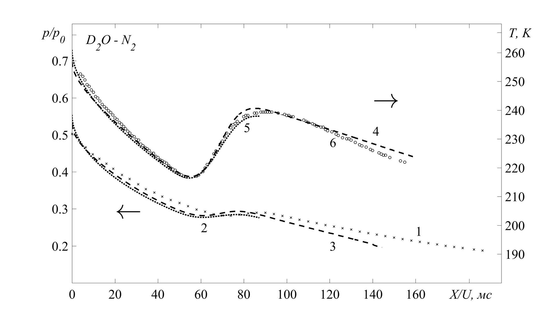
I would like to tell you about the charms of this team by my own example. The task is that I need to build on one graph 3 temperature profiles (solutions obtained by a direct numerical method, a torque method and experimental values) related to the right axis, and 3 pressure profiles related to the left axis. And also add arrows and captions.
The yyaxis left and yyaxis right commands allow you to cope with this task at a time. What, in fact, the essence. Within one figure, we can build any number of graphs, tying them to one of the axes. Within each of the teams, everything works just the same as for regular charts.
The structure of the picture in this case will look like this:
Having filled this structure with necessary, we get as a result:
Another additional feature in preparing graphics for printing is their simple and convenient saving in any format supported by Matlab. To do this, just add the following lines:
Total
Starting with version R2014a, Matlab has become a suitable program for preparing schedules for publishing articles in various scientific journals. An important advantage is the very good flexibility of this tool, which allows you to process the results and present them in a digestible and beautiful form, including for the so-called. "Batch" processing.
This is worth a look:
→ Useful article on graphics in Matlab
→ Description yyaxis
→ Description plotyy
→ Export Graphs
When preparing graphs for publishing articles in scientific journals and various kinds of reports, I often came across the need to construct several curves, each relating to its own axis - in order not to overload the article with graphs and not go beyond their limit. But for this in Matlab, up to version R2014a, there was only the plotyy command (X1, Y1, X2, Y2) , which has a number of unpleasant features that caused other programs to be used and done manually, which, first, complicates this process from the point of view of a unified stylistics, secondly, it requires a large amount of time, and thirdly, it does not allow for prompt changes.
Unpleasant features and description
These unpleasant features I would attribute:
')
1. The lack of an analogue of hold on (“native” hold on does not work quite correctly with plotyy). In order to add more than 2 curves it is necessary to use the following construction:
From this construction follows an unpleasant feature number 2:
2. Dimensions of arrays enclosed in square brackets must match, since from them matrices of elements are formed. In practice, this happens very rarely.
3. The design seriously suffers from the fact that it is impossible to change the colors and types of all lines in a row using software methods; you can format only a set of lines related to a specific axis (hLine1 and hLine2) - in any case, I could not. At the same time, I do not speak now about changing the parameters by hand, editing in the “figure” window - only directly with the code in the .m file.
In summary, plotyy () is not well suited for displaying multiple sets of graphs for different axes. Unless for simple dependencies like these:

')
1. The lack of an analogue of hold on (“native” hold on does not work quite correctly with plotyy). In order to add more than 2 curves it is necessary to use the following construction:
[hAx,hLine1,hLine2] = plotyy([x1',x2'],[y1' y2'],[x3',x4'],[y3',y4']); % 4 From this construction follows an unpleasant feature number 2:
2. Dimensions of arrays enclosed in square brackets must match, since from them matrices of elements are formed. In practice, this happens very rarely.
3. The design seriously suffers from the fact that it is impossible to change the colors and types of all lines in a row using software methods; you can format only a set of lines related to a specific axis (hLine1 and hLine2) - in any case, I could not. At the same time, I do not speak now about changing the parameters by hand, editing in the “figure” window - only directly with the code in the .m file.
In summary, plotyy () is not well suited for displaying multiple sets of graphs for different axes. Unless for simple dependencies like these:
x = linspace(0,10); y1 = 200*exp(-0.05*x).*sin(x); y2 = 0.8*exp(-0.5*x).*cos(10*x); y3 = 0.2*exp(-0.5*x).*cos(10*x); y4 = 150*exp(-0.05*x).*sin(x); X=[x',x']; Y1=[y1' y4']; Y2=[y2',y3']; [hAx,hLine1,hLine2] = plotyy(X,Y1,X,Y2); But the yyaxes team, which appeared in the version of Matlab R2014a. Here we have where to turn.
I would like to tell you about the charms of this team by my own example. The task is that I need to build on one graph 3 temperature profiles (solutions obtained by a direct numerical method, a torque method and experimental values) related to the right axis, and 3 pressure profiles related to the left axis. And also add arrows and captions.
The yyaxis left and yyaxis right commands allow you to cope with this task at a time. What, in fact, the essence. Within one figure, we can build any number of graphs, tying them to one of the axes. Within each of the teams, everything works just the same as for regular charts.
The structure of the picture in this case will look like this:
figure() { - , } yyaxis left { , - , , , } yyaxis right { , - , , , } Having filled this structure with necessary, we get as a result:
Program code
% h = figure('Units', 'normalized', 'OuterPosition', [0 0 1 1]); % : F='Times New Roman'; FN='FontName'; FS='FontSize'; l=30;% set(gca, FN, F, FS, l) box on % hold on %% yyaxis right hPlot_1 = plot(time*10^6, T); % hPlot_2 =plot(time_exp_T*10^6, T_exp); % hPlot_3 =plot(time_pk, T_pk); % set( hPlot_1, 'LineWidth', 3, 'LineStyle', ':', 'Color', 'k' ); set( hPlot_2, 'LineWidth', 1, 'LineStyle', 'none', 'Color', 'k', 'Marker', 'o' ); set( hPlot_3, 'LineWidth', 3, 'LineStyle', '--', 'Color', 'k' ); % () ylim([180 270]); % () yticks([190 200 210 220 230 240 250 260 267]) yticklabels({'190', '200', '210', '220', '230', '240','250' '260', '\it T, K'}) % set(gca,'xcolor','k'); set(gca,'ycolor','k'); %% yyaxis left hPlot_10 = plot(time_P*10^6, P_p0); % hPlot_11 = plot(time_exp_P_p0*10^6, P_p0_exp); % hPlot_13 = plot(time_pk, Pp0_pk); % set( hPlot_10, 'LineWidth', 3, 'LineStyle', ':', 'Color', 'k' ); set( hPlot_11, 'LineWidth', 1, 'LineStyle', 'none', 'Color', 'k', 'Marker', 'x' ); set( hPlot_13, 'LineWidth', 3, 'LineStyle', '--', 'Color', 'k' ); % () ylim([0.1 0.8]); % () yticks([0.2 0.3 0.4 0.5 0.6 0.7 0.77]) yticklabels({'0.2', '0.3', '0.4', '0.5', '0.6', '0.7', '\it p/p_0 '}) % set(gca,'xcolor','k'); set(gca,'ycolor','k'); %% % xticks([0 20 40 60 80 100 120 140 160 185]) xticklabels({'0' '20' '40' '60' '80' '100' '120' '140' '160', '\it X/U, c'}) % text(20,0.3,'\leftarrow', FS, 60, FN, F); text(140,0.6,'\rightarrow', FS, 60, FN, F); text(160,0.24,'1', FS, l, FN, F); text(60, 0.25,'2', FS, l, FN, F); text(120, 0.2,'3', FS, l, FN, F); text(140,0.51,'4', FS, l, FN, F); text(80, 0.52,'5', FS, l, FN, F); text(120,0.48,'6', FS, l, FN, F); text(5,0.75,'\it D_2O - N_2', FS, l, FN, F); hold off Another additional feature in preparing graphics for printing is their simple and convenient saving in any format supported by Matlab. To do this, just add the following lines:
%% file_name = strcat('T, p_p0 - mm, ch, exp'); % saveas(h, file_name, 'bmp'); % .bmp saveas(h, file_name, 'fig'); % .fig saveas(h, file_name, 'eps'); % .eps saveas(h, file_name, 'jpeg'); % .jpeg close(h); % Total
Starting with version R2014a, Matlab has become a suitable program for preparing schedules for publishing articles in various scientific journals. An important advantage is the very good flexibility of this tool, which allows you to process the results and present them in a digestible and beautiful form, including for the so-called. "Batch" processing.
This is worth a look:
→ Useful article on graphics in Matlab
→ Description yyaxis
→ Description plotyy
→ Export Graphs
Source: https://habr.com/ru/post/403763/
All Articles