Gene networks that control the body structure of animals

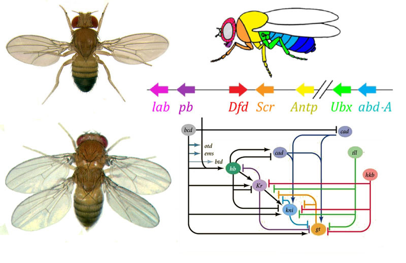
How to turn an egg into a larva and then into an adult fly with the help of gene networks? A fly, like other insects, consists of segments. Segments are combined into three groups - head, chest and abdomen. There may be a pair of limbs on a segment. There are three segments in the chest, each with a pair of legs. The second thoracic segment also has wings, and the third - the halter (small steering wings, almost imperceptible without a magnifying glass). The abdomen consists of eight segments, no limbs on them. Initially, there were six segments in the head, but during the evolution of insects, the boundaries between them were completely erased. Their limbs are the antennae with which the fly sniffs and feels, and three pairs of mouth limbs. In a beetle or cockroach, these would be mandibles, maxillae and lower lip, while in a fly they all merge into a proboscis.

In order for all the organs to be in their place, each cell must know in which place of the embryo it is. Therefore, in the early stages of development of the embryo, when there are still no organs in it and all the cells look the same, a biochemical “coordinate grid” with the anteroposterior, dorsal-ventral and left-right axes appears in it. Mutations of the genes that form the grid can easily and quickly change the appearance of the animal - move the organs to another place, change their number, and so on. Therefore, such genes are important for the evolution of animals and are being actively studied. The gene network of germ markings in Drosophila fly, a favorite toy of geneticists, is perhaps the most studied among animal gene networks.

The algorithm for marking eggs on the anterior-posterior axis is in principle simple:

1) determine which end of the egg will be the head, which tail
2) divide the embryo along the anteroposterior axis into 17 segments
3) divide each segment into front, middle and back
4) mark the head (6 segments), chest (3 segments) and abdomen (8 segments)
5) mark individual segment differences
')
The gene network that does this has a modular device. Each module performs its own step of the general algorithm. Drosophila fly turned out to be a very convenient object for studying gene developmental networks, because it has very bright and significant hereditary deformities. For example, the antennapedia mutation, in which the antennae turn into legs, or the VTHROMMANNERS proboscipedia, when part of the trunk is turned into legs. The bithorax mutation gives a four-winged fly, which, in addition to the usual wings on the second pectoral segment, has a second pair of wings on the third pectoral segment.




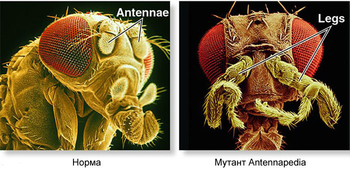
Such mutations, in which one part of the body becomes very similar to the other, are called “homeotic”. Starting with these mutants, genetics eventually deciphered the entire network of genes that control the development of the fly. This work won the Nobel Prize in 1995.

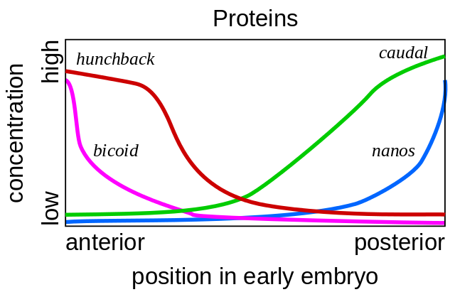
It all starts with the genes of the polarity of the egg - bicoid and nanos. They work even before the fertilization of the egg, while it matures in the mother’s ovary. Auxiliary cells pumping nutrients into the egg are located on one side of it, so the egg has two different ends from the very beginning. Bicoid matrix RNA accumulates at the front end of the egg, where it is fixed and cannot swim away. Nanos mRNA is similarly fixed at the posterior end. After fertilization, proteins are synthesized using these mRNAs. Their molecules spread through the egg. Since bicoid and nanos proteins are synthesized at one end of the egg, and decay is everywhere, a bicoid gradient of the protein, which decreases from the front end of the embryo to the back, and the nanos gradient from the back to the front end are obtained.



If a bicoid mRNA is introduced with a micropipette to a different location of the egg, a second head will grow there. If you artificially turn off the bicoid mRNA, you get a fetus without a head and with two asses.
Next, the bicoid and nanos proteins include the genes of the embryo itself, that is, new mRNA begins to be read from them). The genes of the gap group are the first to start working, from the English gap - the gap. The first two genes of this group, hunchback and caudal, form gradients from head to tail (hunchback) and from tail to head (caudal). But their gradients are smoother than bicoid and nanos.


The remaining four genes of the gap group each form one or two wide (more than one segment) bands with fairly clear boundaries. They are incorporated by upstream protein products (bicoid, nanos, hunchback and caudal). A complete shutdown of one of the genes of this group gives a shortened embryo, which lacks several segments, in which this gene normally worked.


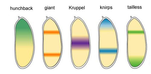
Gene activity areas of the gap block

Why is it that the four genes of the gap block (kruppel, giant, knirps and tailless) divide the embryo into bands, each of which runs one of the four genes?

First, they all inhibit each other's activity. In a single cell, there would be a steady state in which one gene from such a group actively works and suppresses all the others (trigger). But the developing egg of a fly is more complicated. In it at this moment in the common intracellular fluid (cytoplasm) thousands of individual cell nuclei float. Egg sizes are large enough so that the rate of breakdown of regulatory proteins is comparable to their diffusion rate at the other end of the egg. With a combination of diffusion and mutual suppression, another steady state appears when the egg is divided into several bands, in each of which one gene from the group works. The slower the diffusion of proteins or the faster the breakdown, the smaller these strips or spots will be. The participation of such systems (they are called reaction-diffusion) in the marking of the body of animals was predicted by Alan Turing (yes, who invented the “Turing machine”) in 1952. At that time, little was known about genes and proteins, but the equations describing striped and spotty structures were correctly derived by Turing. Here or here you can play with a simple reaction-diffusion model of two substances and experience how it can behave.


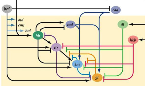
Connections between gap genes and egg polarity genes. Bcd - bicoid, hb - hunchback, cad - caudal, Kr - Kruppel, kni - knirps, gt - giant, tll - tailless.

In itself, the suppression of each other's genes will mark the embryo into some strips, but the arrangement of the activity strips of the four genes relative to each other and the ends of the embryo will be very variable. In order for the stripes to always be in place (for example, for knirps, one strip in the head, the other in the back half between the kruppel and giant stripes), a second control signal is needed — bicoid gradients and other egg polarity proteins. The input functions of the gap genes for these regulators have maxima at different input signal levels (we derived such an input function at the end of the second article ). Therefore, gap genes are each included in their level of bicoid, hunchback and caudal proteins, and their activity zones are regularly located from the head to the tail of the embryo.

After the gap genes have done a rough marking of the embryo into 7 lanes (they do not coincide with the segments, nor with the head-breast-abdomen), the following module is included - pair-rule (“pair rule genes”). It divides the embryo into segments, which should be 17. The pair-rule module consists of five genes, and all of them, as you might have guessed, suppress each other. Each of these genes works either in all even or in all odd segments — the proteins they encode break down faster than the proteins of the gap group, and the stripes are correspondingly narrower. Turning off part of the genes of this group gives a shortened germ, in which all even or all odd segments disappear.


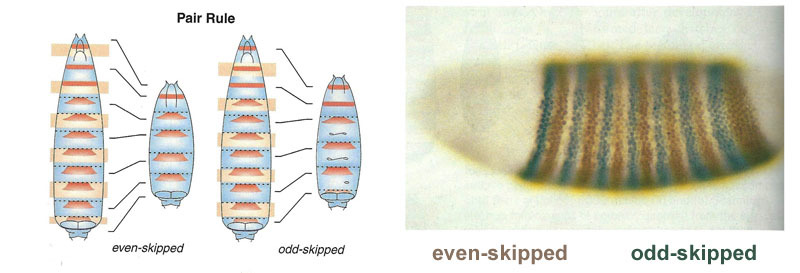
Zones of activity of genes from the pair-rule group. In the photo there are 14 stripes on the right, not 17, because in the first three segments of the head, another marking system works.

The pair-rule module itself, without the participation of gap and bicoid, can mark the embryo into narrow strips, but the number of these strips would be unstable: the segments can turn out to be 12, and 18, and even 20. Normally, the pair-rule genes are difficult to manage. gap genes, and the first rough markup (in 7 zones) helps to accurately and reliably make the final markup (in the 14 + 3 segments).

The next point of the algorithm is to mark the front, middle and back of each segment. This is done by segment polarity genes. They also suppress each other and are switched on by higher-level modules of the network gene (pair-rule and gap). Only the diffusion and decay parameters of their products are chosen so that the strips are very thin - half the segment. Suppressing them with each other is weaker and more complicated than the pair-rule genes. Therefore, their activity strips partially overlap, and in each segment there is a frequent “ruler” of different overlapping strips.

Switching off segment polarity genes usually does not lead to shortening of the embryo and loss of its parts (as is typical for gap and pair-rule), but to more subtle effects. Usually, half of each segment in which this gene should work turns into a mirror image of the other half. This is clearly visible, because the fly larva has rows of small spines directed backwards - for ease of crawling. In mutants on segment polarity genes, rows of spinules appear, directed forward.

Finally, it is the turn of the most famous and first-discovered genes of this network - the hox module. Their work gives the segments individuality so that the antennae and proboscis grow on the head segments and the legs and wings on the thoracic segments. The hox genes, unlike the previous modules, do not inhibit each other's activity and can work together in the same germ segment. A strange property of the hox genes, which has not been explained so far: they are located in the chromosome in a close group, and in the same order in which they work in the body of the embryo.



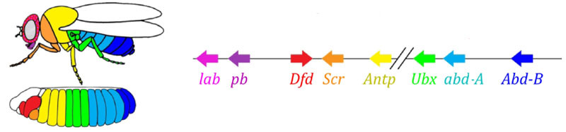
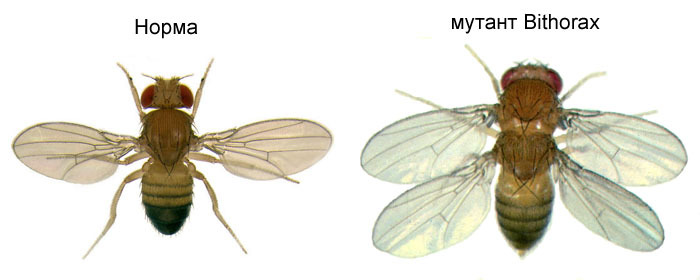
Embryo marking is arranged according to the principle “the farther from the breast, the more hox-genes and the more active it works”: abdominal-A gene activity starts from segment 2 of the abdomen, increases to full in 4 and continues at the maximum level in all subsequent segments; The abdominal-B gene works from 5th to 8th abdominal segment, increasing activity in each next segment. The ultrabithorax gene is activated at half strength in the third thoracic segment and at full capacity around the abdomen. When it is turned off in the mutant bithorax, cells of the 3rd thoracic segment do not know that they are the 3rd thoracic segment; Program 2 thoracic - with wings instead of a buzzard and powerful flying muscles.

If you turn off all the hox-genes in a separate segment, it will turn out to be ugly, but it will be most similar to 1 chest, with legs and without wings. This is because the distant ancestors of the insects were like trilobites or centipedes. They had many identical segments with legs. Subsequently, their body was shortened, the back part lost its legs, becoming abdomen, and several front segments joined the head and their legs became parts of the mouth apparatus (mandibles, maxillae, and lower lip).

Mathematical models of the germ markup gene network

In the case of the lactose operon and loops of the direct connection in E. coli, it is possible to construct fairly simple mathematical models with a moderate number of parameters that predict the behavior of genes in any input signals. For the lactose operon is enough:

- four binding constants (repressor and activator with DNA, lactose with repressor, cAMP with activator)
- four parameters of stoichiometry (4 lactose per 1 repressor, 2 cAMP per 1 activator, 1 repressor each and activator per operon)
- two parameters of regulation (the effect of repressor and activator on the probability of landing of RNA polymerase)
- the basic level of operon activity (when there is no repressor or activator)
- transcriptional delay
Total 12 parameters.

Now let's look at the regulatory regions of, say, the Hox genes. In the diagram below, one of the regulatory blocks of the abdominal-B gene.



The colored bars indicate the binding sites of the regulatory protein. This entire block is about 1,700 nucleotides in size - 10 times longer than the regulatory region of the lactose operon. It has 39 landing sites for 7 different regulatory proteins from all the higher blocks of this gene network. And abdominal-B has four such regulatory blocks. They are included in sequence from abdomen segment 5 through 8 and create a stepwise increase in abdominal-B protein level in these segments. That is, for the matmodel of one of this gene, in an amicable way, more than 100 binding constants, the same number of regulation parameters, and an unknown number of parameters are needed to describe the interaction between different inputs - in the worst case, up to one and a half thousand for pairwise interactions between all protein landing sites in one regulatory block. That is, the complete model of this gene network will obviously have more than a thousand parameters. And this is the main problem: there are not so many output signals that we can measure in the experiment - in fact, only the levels of each of the 25 proteins and their distribution along the length of the embryo. Therefore, no one even tried to model this network with the same detail as the lactose operon.

You can try to simplify the task and describe the effect of each regulatory protein on a gene with only three parameters (binding, stoichiometry and regulation parameter). You can choose these parameters (for example, using Markov chains) so that the model accurately reproduces the real bands of gene activity. For the first two blocks of the network (egg polarity genes and gap genes), such models are even made ( for example ).

The problem is that different starts of the selection algorithm give different parameters of the model - but they all work correctly and reproduce the activity of genes in a real fly germ! These models have common features (for example, all gap genes suppress each other and are activated by maternal proteins), but the differences are no less than similarities.

And since different modeling attempts give different results, it is unlikely that at least one of them coincides with reality. Worse, such models reproduce normal work, but miss the mark in predicting the results of mutations.

In the next part we will talk about why these troubles with the study of gene networks are inevitable in biology (and the Drosophila germ markup network is one of the simplest ones to learn!), What can be done about it, and what engineers should biologists learn from.