Intermodulation Distortion in Audio and OOS Amplifiers - Caution, Dangerous Connections

On audiophile sites, it is customary to frighten visitors with intermodulation distortions, however, since most publications on this topic make extensive use of copy-paste technology, it is hard to understand why these distortions arise and why they are so scary. Today I will try, to the best of my abilities and the volume of the article, to reflect precisely the nature of these pages.

The topic of signal distortion in the UMZCH was raised in my previous article , but last time we only slightly touched linear and non-linear distortions. Today we will try to understand the most unpleasant to the ear, elusive for analysis and difficult for designers of ULF intermodulation distortion. The reasons for their occurrence and the relationship with the feedback sorry for the pun .
')

Operational amplifier as a white triangle

Before we talk about feedback, we will do a little excursion into the operational amplifier OU , since today the transistor amplifying circuits practically do not do without them. They can be present in the form of separate microcircuits, as well as be part of more complex chips — for example, low-frequency integrated amplifiers — ULF .

Consider the amplifier in the form of a black box or rather a white triangle, as they are usually denoted in circuit design , without going into details of its device.

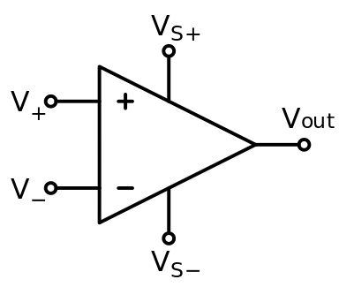
Pin assignment of an operational amplifier

Non-inverting input:

Inverting input:

Plus power supply:

Power supply minus:

If we increase the input voltage at a non-inverting input, then the output voltage will increase, if at the inverting input, the opposite will decrease.

Usually, the input voltage that needs to be amplified is supplied between two inputs and then the output voltage can be expressed as follows:

Where - gain with open loop feedback

Since our goal is not to amplify constant voltages, but to sound vibrations, let us consider, for example, the dependence low-cost op-amp LM324 on the frequency of the input sinusoidal oscillations.

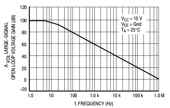
In this graph, the gain is plotted vertically, and the frequency is on a logarithmic scale horizontally. The results of the work of engineers are not too impressive and it is unlikely that this amplifier can be used in reality. First, it shows good linearity only outside the frequency range perceived by the ear - below 10 Hz, and secondly, its gain is too large - 10,000 times at a constant current!

So what to do, there must be a way out! Yes, he is. Take part of the output signal and feed it to the inverting input - enter feedback.

Feedback is simple and angry! Panacea for all ills?

In this article we will not touch on the basics of the theory of operational amplifiers, if you wish, you can find a lot of information on this topic on the Internet, for example, in the cycle of articles by Igor Petrov KriegeR

Entering feedback into the amplifier circuit is not easy, but very simple. Let's not go far to see how this can be done using the example from my last article about the little tricks of tracing circuits on operational amplifiers .

Feedback in this circuit is fed to the inverting input of the shelter through a resistor R2, more precisely a voltage divider from R2 and R1.



It is easy to prove that this circuit will have a voltage gain equal to two, and it will be unchanged when amplifying harmonic signals in a very wide frequency range. With an increase in the signal frequency, the gain of an op amp without an operating system drops, but remains many times more than two, and this drop is compensated for by an automatic decrease in the feedback signal level. As a result, the gain of the circuit as a whole remains unchanged. But that's not all. This circuit has a very high input impedance, and therefore has virtually no effect on the signal source. It also has a very low output impedance, which means, in theory, it should retain the shape of the signal even when operating at a sufficiently low impedance load, and with complex impedance — inductive and capacitive.

Have we really got an IDEAL AMPLIFIER like that?

Unfortunately, no, as any coin has an eagle and tails, and feedback has its dark side.

What is good for a Russian, a German is death or some radio engineering

In radio engineering, the effect of the interaction of signals from two different frequencies applied to a nonlinear element, called intermodulation , is well known. The result is a complex signal with combinations of frequencies (harmonics) depending on the frequency of the original signals f1 and f2 according to the following formula:

The resulting frequencies in amplitude are less than the parent harmonics and, as a rule, their level rapidly decreases with increasing integer coefficients m and n.

The greatest amplitude will have harmonics, called second order harmonics with frequencies:

and third order harmonic frequencies:

In radio engineering, this effect is widely used for frequency conversion. Thanks to him, modern receivers work. Frequency conversion occurs in mixers, built on the basis of nonlinear elements as which often use the pn junction diode, well, or a transistor. The mixer simultaneously receives the received signal and the signal from the oscillator - the local oscillator.


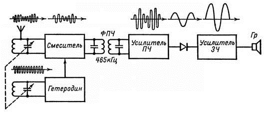
At the output we get a wide range of signals:


But thanks to the narrowband filter of the FPC, we select the signal we need with an intermediate frequency f _pr = f gf and amplify it in the IF amplifier. Then there is a detection using the following nonlinear element, usually a diode and the output after the low-pass filter is not shown in the figure, we receive an audio signal.

IMI (IMD) - intermodulation distortion

However, if the intermodulation effect is vital for receivers, in low-frequency amplifiers, it causes non-linear distortions, which are called intermodulation. After all, the sound signal simultaneously contains harmonics of a large number of frequencies, which differ greatly in amplitude, and the transistors that make up the amplifier, like diodes, are nonlinear elements. The distortions that appear due to the mechanism described above in the English-language sources are called intermodulation distortion abbreviated IMD , by the way the Russian abbreviation for them is THEM .

This type of distortion is much more unpleasant to the ear than the banal amplitude limitation of the signal, the source of their appearance in each particular case is much more difficult to detect and, most importantly, eliminate.

Fight this effect by applying more advanced transistors operating in a linear mode and using local amplification within one cascade or deep general feedback - a jack of all trades! However, everything is good in moderation - if the frequencies of the parasitic harmonics of the signal lie in the region of the rapid decline in the amplitude-frequency characteristic of the amplifier, the feedback may not have time to compensate for signal distortion and even itself cause a source of additional distortion.

It's time for us to finally get into the dark side of feedback.

The dark side of feedback

In order to detect it, we will assemble an amplifier according to the scheme presented above at the LM324 op amp, but with slightly different feedback resistor nominal values ​​so as to obtain a single gain.

And now we give a small amplitude square pulse at its input, some 100 millivolts.


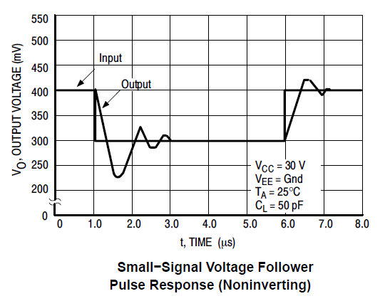
What we got at the output does not look like an input signal. What happened and why didn't the feedback help us? As always, physics is to blame; its world is much more complicated than our mathematical models based on rough approximations. The fact is that our amplifier is a very complex device.



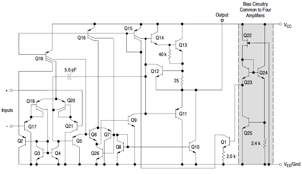
It contains a lot of parasitic capacitances located both inside the integrated transistors, its components, and in interstage connections. The nature of parasitic capacitances is very different, for example, due to the resorption time of minority charge carriers in a semiconductor. The transistors themselves, on which our op amp is built, are amplifying devices with high non-linearity. Moreover, the elements of the printed circuit board have their own capacity, especially if the trace did not take into account the recommendations set forth in my previous article .

At the moment of arrival of a negative signal front, the feedback detects that the input voltage does not correspond to the output one. It dramatically increases the potential of the inverting input with respect to the non-inverting input in order to transfer the voltage surge at the amplifier input as quickly as possible, but it does not have time to do this because it needs to charge the parasitic capacitances of the entire amplification path first and we get the edge of the output signal. Further, when the input signal also abruptly ceases to change the feedback is forced to discharge these capacities. As a consequence, we get an output burst, which later turns into a damped oscillatory process. In especially sad cases, this oscillatory process can be delayed for a rather long time - the amplifier will go into a state of self-excitation. As a result, new harmonics that are not present at the input appear in the signal at the output of the amplifier — nonlinear distortions.

Excursion to the real world. General negative feedback in the audio power amplifier

The nonlinearity inherent in transistor cascades forces developers to use strong negative feedback as the simplest solution for fitting amplifier parameters to meet the requirements for low harmonic and intermodulation distortion of course measured by standard methods . As a result, industrial power amplifiers with an EP of 60 or even 100 dB are not uncommon today.
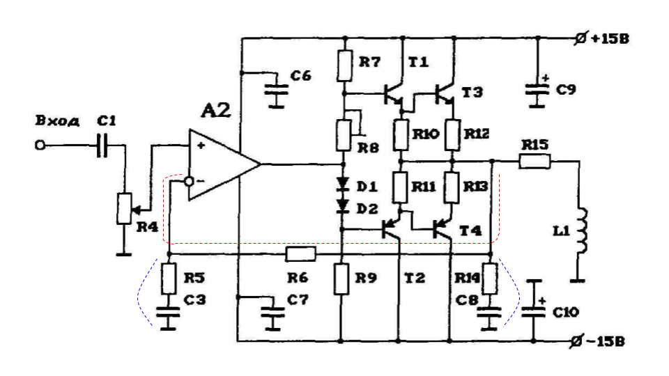
Let's draw a real circuit of a simple transistor power amplifier. We can say that it is a three stage one. The first amplifier stage on the op amp A1, the second on the transistors T1-T2 and the third transistor T3 -T4. In this case, the amplifier is covered by a common feedback circuit , it is highlighted by a red circuit , which is fed through a resistor R6 to the non-inverting input of an op-amp. The key word here is common - feedback is fed here not from the output of an op-amp to its input, but from the output of the entire amplifier.



As a result, due to its enormous amplification, the op amp should help to cope with different kinds of non-linearities and noise in transistor amplifier stages. Here are the main ones:

• transistors in such a connection can operate in a very non-linear mode when the signal passes through zero and for weak signals;
• at the output of the amplifier is loaded on a complex load - speaker system. The diagram shows its equivalent - resistance R15 and inductance L1;
• Transistors operate in heavy thermal conditions and the temperature of their body substantially depends on the output power, and their parameters strongly depend on the temperature;
• Capacities of mounting and various kinds of pickup can have a decent value and trace errors can easily lead to the appearance of positive feedback and self-excitation of the amplifier;
• Significantly increases the role of interference induced on power;

And OU helps, but as a fool, praying to a god of a famous aphorism is sometimes too hard. There are problems with the overload capacity of individual cascades, the transistors of which fall into the signal limiting mode. They go from a linear course of a relatively linear mode to cut-off or saturation modes. They leave very quickly, and return to it much slower, which is caused by the slow process of resorption of minor sources of charge in semiconductor transitions. Let us consider this process and its consequences in more detail.

TIM Dynamic Intermodulation Distortion. Overload capability and amplifier clipping effect

The overload capacity of an amplifier is a parameter that describes how many decibels the nominal output voltage or power differs from the maximum when the output signal limits on power start - clipping

In transistor amplifiers overload capacity is small, especially in the terminal and pre-terminal cascades. Rated power from the maximum often differs by only 40 percent, which is less than 3 dB.

Imagine that our amplifier consists of an ideal preamplifier of a corrector and a UMFR covered by feedback with a factor B. It is important to note that the signal V ₁ may contain components of a very high frequency. Preamplifier C acts as a low-pass filter, producing an input signal V ₂ for amplifier A, containing only components that fall into the sound frequency band.



The voltage at the input of the power amplifier V ₂ has a rise time determined by the preamplifier, the graph shows that it is smoothed. However, in the voltage V ₃ , acting at the output of the adder, there is an outlier, caused by the desire of the feedback to compensate for the low speed of the power amplifier A with the amplitude V _max


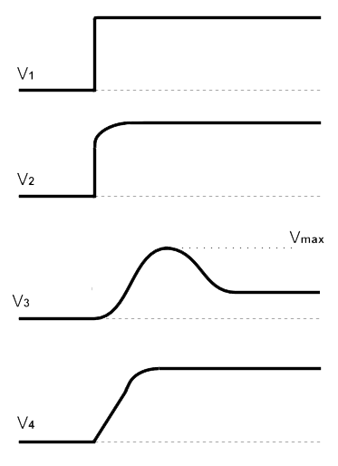
The emission in the signal V ₃ can be hundreds or even thousands of times greater in amplitude than the nominal level of the input signal. It can greatly exceed the dynamic range of the amplifier. During such an overload, the gain of other signals present at the input decreases, causing an instantaneous surge in intermodulation distortion. This surge is called dynamic intermodulation TID distortion , because it leads to the influence of one signal on the amplitude of another intermodulation , and depends on the time and amplitude characteristics of the input signal more than just the amplitude response, as in the case of simple intermodulation distortion.



In the shown circuit, the voltage gain has the greatest gain, however, it has a good overload capacity - it retains small non-linear distortions with the voltage swing at the output close to the supply voltage. The situation is much worse with the cascade on the transistors T1 and T2 - these are current amplifiers that can be simply removed from normal operation, and it may take a relatively long time to restore it. The overvoltage feedback voltage gains of op amps and input to these transistors can have very large values. They overload the second amplification stage. T1 and T2 can enter saturation mode, lose their amplifying properties, and remain in it for some time even after the abrupt front of the input signal disappears, until the charge dissipates on various kinds of parasitic capacitances. Parasitic capacitances and possible elements of the correction of the frequency response here are shown using the elements R and C.


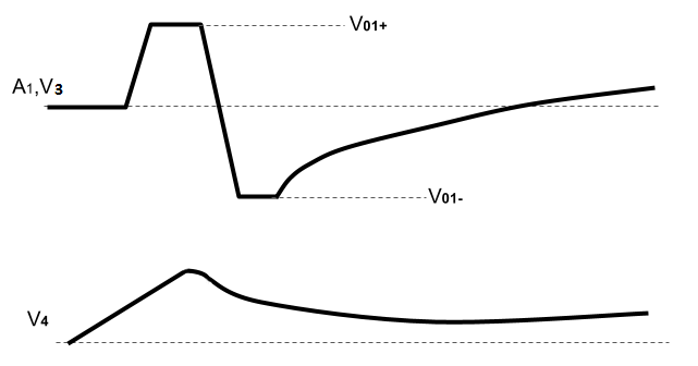
Above is a graph of an extremely unpleasant effect, which is called “clipping” the amplifier and it is the result of feedback. At the output of A1, we get the effect of amplitude limiting, and at the output of the amplifier a distorted signal.

Methods of measuring intermodulation distortion and methods of dealing with them

According to the standard method for measuring intermodulation distortion, two signals are simultaneously fed to the input of the object being measured: low f ₁ and high f ₂ frequencies. Unfortunately, in different countries use different measuring frequencies. Different standards provide different frequencies - 100 and 5000 Hz, 50 and 1000 Hz ...

The most common is the use of frequencies of 400 and 4000 Hz, approved in DIN 45403, GOST 16122-88 and IEC 60268-5. The amplitude of the signal with frequency f ₁ by 12 dB is 4 times greater than the amplitude of the signal with frequency f ₂ . Depending on the nonlinearity of the characteristic, differential and total combination oscillations f ₂ ± f ₁ and f ₂ ± 2f ₁ higher orders of magnitude are formed symmetrically with respect to the frequency f ₂ . The resulting combination oscillations of the second order with frequencies f ₂ ± f ₁ characterize quadratic, and the third order with frequencies f ₂ ± 2f ₁ - the cubic distortions of the measurement object.

A pair of frequencies of 19 and 20 KHz is also widely used, with an equal signal level, which is convenient primarily because the main harmonic that falls within the sound range, in this case, is a signal with a frequency of 1 KHz, the level of which is easy to measure.

Not only generators are used to supply measuring signals, but also measuring CDs and even vinyl records specially recorded in the studio.


About 30 years ago, complex and expensive instruments, available only in laboratories and studios, for example, the composition of the measuring stand for the pickup amplifier, were required to measure the intermodulation distortion factor:

1. Vinyl record player;
2. Measuring plate;
3. Pickup;
4. Correction amplifier;
5. Bandpass filter;
6. Linear detector;
7. Low pass filter.
8. And of course V is a voltmeter that can measure the effective value of sinusoidal oscillations!

Today, even a simple 16-bit computer music card with a price of up to $ 30 complete with a special measurement program and simple matching circuits can provide much better measurement quality.

The described standards are very convenient for manufacturers of audio reproducing equipment , you can easily get beautiful small numbers in the passport data , but not very well reflect the real quality of the amplifier path. The result, of course, is the development of subjectivism - when two amplifiers or even expensive audio cards with formally almost identical parameters “sound” completely differently on a complex musical signal — you cannot do without listening before you buy.

Fans of high-quality sound enthusiasts and individual manufacturers of high-end equipment manufacturers are trying to promote their measurement techniques based on less approximating from reality. There are multifrequency techniques, techniques investigating the interaction of the harmonic frequency and a single pulse, based on noise signals and others. However, this time we will not have time to discuss them in detail.

We will also dwell briefly on the methods of dealing with intermodulation distortion:

• Adjustment of circuitry with the aim of obtaining good results for standard measurement techniques;
• Frequency - dependent feedback and frequency correction chains of the R5, C3 and R14, C8 chains in the picture in this article ;
• The use of local feedback chains covering one to two amplification stages;
• The introduction of transistors in the linear mode. In our picture of the amplifier diodes D1, D2 and trimmer R8 are responsible for this. However, this measure is fraught with increased energy consumption, especially the output stages;
• The use of high-quality and expensive components;
• Finally, the most radical is the use of lamps instead of transistors as more linear elements. However, this is a separate large and ambiguous topic worthy of a separate article ...

---

Perhaps this is my last article this year, taking the opportunity to wish all my readers a Happy New Year and wish happiness and good luck in the coming!