The 2008 Financial Crisis: Causes and Effects
In 2008, when the market collapsed, I was a 16-year-old young man who first visited London. By that time, I was already obsessed with finances. Being sure that after reading classic books like “Analysis of Securities”, “Reasonable Investor” and “Ordinary Shares and Extraordinary Revenues”, I can understand the reasons for what happened, I bought the Financial Times issue and plunged into the newspaper lines. True, then I understood little. Each paragraph contained questions, not answers. What are "quanta" and "credit derivatives"? And the "securitization"? What does insurance have to do with the stock market? Why has the collapse of the derivatives market affected everything else so much?

The shock of meeting reality opened my eyes. The market is a complex adaptive system, within which are models and computer algorithms that almost no one understands. How can you not remember the words of Gordon Gekko from "Wall Street 2: Money does not sleep": "They call with different names multi-billion loans: CMO, CDO, SIV, MBS. I believe that only 75 people in the world know what it is. ”
Trying to understand and understand, I read books, studied programming, in the end I became the very “quant”, quantitative analyst, whose title did not cause anything but confusion before. Here is my vision of the financial crisis. I do not presume that my conclusions are the ultimate truth, but I rely on reliable data sources. My point of view was influenced by many books and articles read. Among them - “The big game for a fall”, “Quanta. Like math wizards, they earned billions and nearly collapsed the stock market, The Greatest Trade Ever, The Crisis of Crowding, Models Behaving Badly, and A Colossal Failure of Common Sense.
')
In fairness, it must be said that the financial crisis was caused not only by the collapse of credit derivatives. The cause of the crisis is a combination of many interrelated factors and problems. There are risks of bad faith, and illiterate economic policies, and deregulation of the financial sector. Excessive confidence of market participants in the used quantitative models, problems in insurance, too high level of use of borrowed funds on the stock exchange, availability of cheap money in the form of a loan and dangerous assumptions regarding market dynamics made a significant contribution to the development of the crisis. All of these factors, which I will discuss in more detail later, created a self-reinforcing model and led to a huge bubble in the market for credit derivatives. When it broke, the indirect connection of the markets, caused by the large leverage available on the stock exchange, led to a fall in the stock market.
I have divided the article into several sections, each of which gives a detailed account of why a particular factor caused the crisis. However, it is not necessary to read the sections sequentially. You may be returning from the next section to the previous section to assess the interdependence of factors. All the data I used to build graphs can be found on Quandl.com . In particular, from there I took information about interest rates and the real estate market in the USA. I used the data from Sifma.org to obtain data on credit derivatives issued, including credit default swaps (CDS) and debt collateral bonds (CDO).
Risks of bad faith can occur in any situation where someone involved in a risky event knows that he is protected from loss, and someone else will cover the possible costs.
In my opinion, such a shift “from a sore head to a healthy one”, which occurred in mortgage lending, and led to a collapse. And this process itself, securitization, consists in transferring the risk from the lender to the investor by issuing securities that are secured by mortgage debt.
Mortgage banks issued to the borrowers a lump sum of money needed to buy a home in exchange for the borrower's obligation to repay the loan for 15-30 years, taking into account the appreciation rate (that is, with the interest of the bank).
There are two fundamentally different approaches to calculating the rate. The first is fixed. In this case, you can fix the amount of payments. The second is floating. With this approach, the loan rate may fluctuate over time. For example, if the bank believes that the risk of default or non-payment of a loan (say, you have delayed payment) increases, the bank may raise the rate. The same can happen if the central bank raises. That is, the higher the risk of default on the loan, the higher the rate on it. However, at that time everyone had a positive attitude, the rates were falling, so people more often took a mortgage with a floating rate, hoping for its decline in the future and not worrying that they can easily remain without work and cannot even at the minimum rate , pay the debt.
From the point of view of the creditor bank, the risk of default on a loan is on its balance sheet, so it has an incentive to issue as many mortgage loans as possible with the aim of earning more money in the future. From the point of view of the recipient of the loan, the interest on the loan is not as big as the prospect of an increase in the cost of housing that will pay back the interest rate. Except, of course, a situation where the lender is not knowingly going to repay the loan. This is the so-called strategic , planned default. Oliver Wyman conducted a study in 2009 and found that 20% of all defaults in 2008 were just that, and many of them were related to business lending.
Mortgage behaves in the same way as bonds, since the recipient of the mortgage is calculated on it every month, and, as a rule, does not allow default. The main difference between mortgages and bonds is that, as a rule, interest on mortgages is higher than on bonds, because housing prices, under the influence of rising demand, are growing rather quickly, and a loan, at least formally, is issued only to people with a good credit history. and rating, which reduces the likelihood of default on their part. At the same time, mortgage banks get a good profit.
The profits that mortgage banks received attracted the attention of experienced investors who invented the process of securitizing mortgage loans. This process allowed financiers to create a security whose payback was tied to monthly mortgage payments.
At first, the system worked quite well. If we explain this in a nutshell, the mortgage debt that was given to a particular borrower was transferred at a premium to the bank, which packed a lot of such loans into a security, and then sold it at a premium to investors under the guise of a reliable investment. And investors were happy to get a paper on which they received a coupon yield every month. Moreover, this approach has allowed mortgage banks to free up capital and issue more and more loans.
Such debt securities were given various names. For example, mortgage backed securities (MBS's), OBI - collateralized mortgage obligations (CMO's) and OBL - collateral debt obligations (CDO's). Some of these securities included not only mortgage debts of individuals, but also commercial mortgages, car loans, there was even credit card debt and much more. There are many subtleties associated with the process of securitization, which, unfortunately, are beyond the scope of this article. This is better to read on Wikipedia .
At first, the effect of the new debt securities was simply explosive. Turnover of mortgage banks has increased many times (this means that more people were able to buy houses), while banks resold debts to investors, who, in turn, received an investment instrument that brought more income than bonds at the same risk. However, with the spread of securitization, there was a problem, which was that the growth of new high-quality borrowers could not be infinite. It was here that the very risks of bad faith came into force - the mortgage borrower standard was falling.
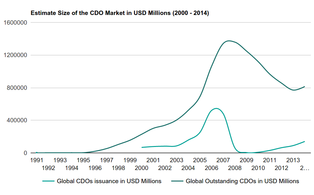
Fig. 1. CDO market size in millions of US dollars
In order to meet the demand for new mortgage loans, lenders lowered standards of requirements for borrowers and began to lend to unreliable private clients, increasing the level of risk. New mortgage companies have entered the market. In particular, it has become popular to issue a floating rate mortgage to customers with a bad credit history and low reliability rating. Banks began issuing mortgages to several houses and low-income people at once. It all worked because the rates were artificially low, and housing prices were constantly rising. But as soon as that changed, the house of cards collapsed. People could no longer afford a monthly mortgage payment, an avalanche of defaults went. Purposeful defaults have also been added to them, since the cost of housing has fallen lower than the cost of the mortgage (often even without interest).
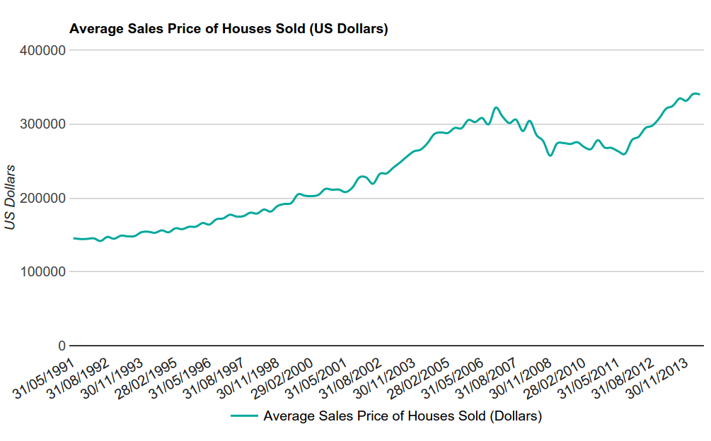
Fig. 2. The average price of homes sold
The above chart reflects the average selling price of a home in the United States, which is published quarterly. The graph shows that housing prices peaked at the end of 2006, and then began to fall, causing an increase in non-payments.
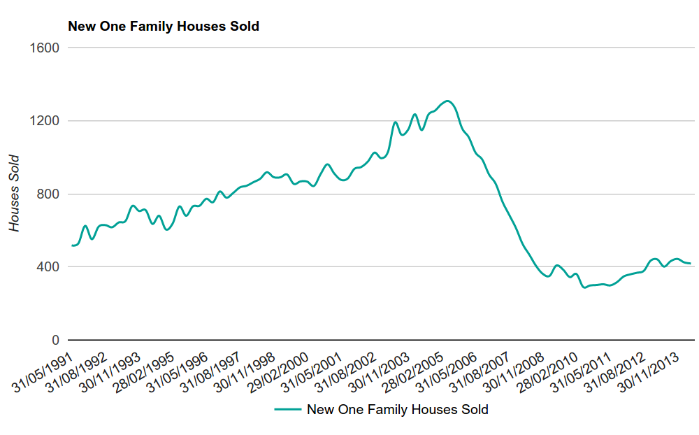
Fig. 3. Demand for new private homes
The above chart shows the demand for new private homes in the USA. Demand in 2006 began to fall. Most likely, this was the reason for the decline in real estate prices.
As already mentioned, artificially low interest rates set by the Fed contributed to the financial crisis. The reason for this was the previous crisis, which occurred when the dot-com bubble burst. Then the Fed lowered the rate to stimulate economic growth. Low rates remained for a very long time. This was a period when many mortgage borrowers took out a loan with a floating interest rate, because they believed that the rates would remain low always, which means that payments would be low. As a result, loans were taken even by those borrowers who could not afford them, and the banks, knowing that the client did not have the means to pay the mortgage, still issued loans, following the strategy of predatory lending .
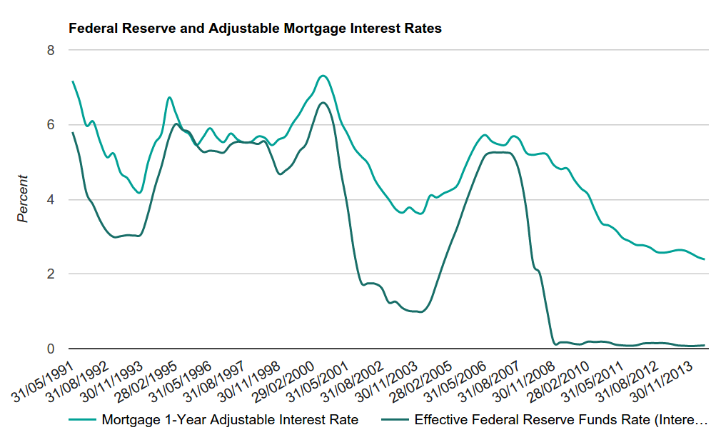
Fig. 4. Floating lending rates
Interest rates represent debt service costs. When interest rates are low, debt service is cheap, and when interest rates are high, debts are expensive. The interest rate on the mortgage depends on the policy and interest rate of the Fed. So between 2004 and 2006, when the Federal Reserve increased interest rates, this led to an increase in mortgage rates. Many homeowners could no longer afford the monthly loan payments and began to purposefully declare defaults on the mortgage. This has not happened before.
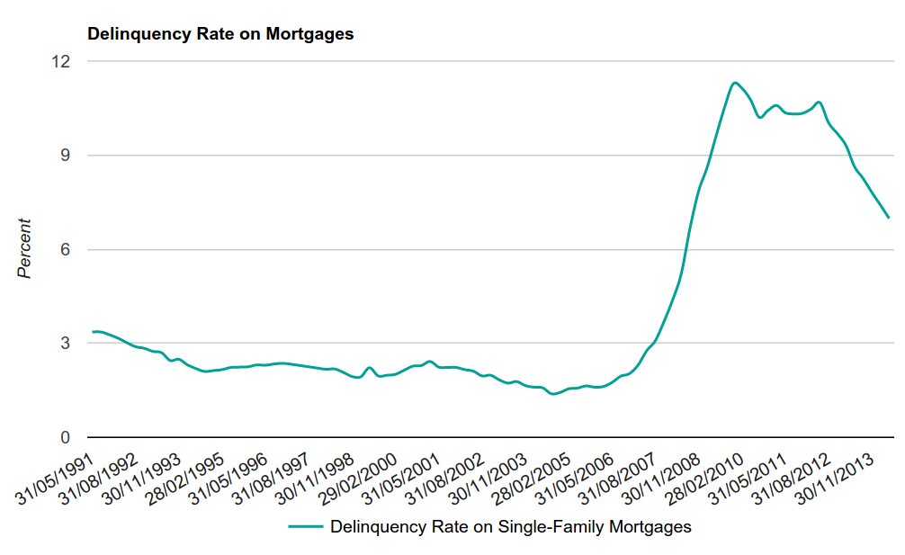
Fig. 5. The share of loans with overdue payments
In each case of delay , the borrower has a certain period for repayment of the debt, then the lender can start a hearing on the rejection of the right to purchase housing and put it up for auction. This is what the average percentage of property alienations per 10,000 houses looks like according to data taken from here .
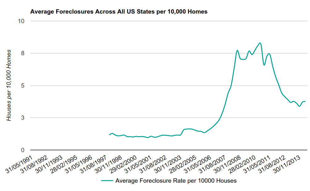
Fig. 6. The average percentage of property alienations for 10,000 homes
So, why did mortgage borrowers default? Here a combination of two factors worked. First, the average price of housing began to fall due to the fact that demand fell, and this spurred targeted defaults on mortgages, since the cost of housing was less than the cost of the loan. Secondly, the increase in mortgage rates put many borrowers in a difficult position, as they lost the ability to repay the loan and were forced to default.
However, the problems with loans alone could not cause a financial crisis. Next, we will discuss other factors that caused the crisis.
The use of quantitative models in finance has become almost ubiquitous, but it seems to me that very few of those who use these models understand the assumptions, initial assumptions, on which the models are built. “Modeling risk” is a term that I coined for this article, which means using a model to solve a problem without understanding the assumptions and limits of model applicability. In this section, I will discuss the use of a Gaussian copula to assess the correlation of credit defaults, and then make a small digression to talk about why machine learning today, in fact, is used incorrectly. Here you can read details about the sources of risk modeling.
Before we delve into the details of the Gaussian copula, the multidimensional distribution function, it is worth noting two fundamental postulates of modern portfolio theory. First, the unsystematic risk of the portfolio is less than or equal to the weighted sum of the unsystematic risks of each individual asset in the portfolio. Secondly, the level to which the unsystematic risk of a portfolio is reduced depends on the interdependence between the assets that make up the portfolio. In other words, by combining assets with a low level of correlation, we can build a portfolio that is less risky than individual assets. This approach is known as diversification.
Given this fact, and combining several credit derivatives, each of which is at risk of default, we will create a portfolio with a lower default risk than each of the tools individually. In other words, we can reduce the risk of credit default through diversification. At the turn of the millennium, the main question was how much diversification reduces risk. The answer to this question was a quantitative modeling method that demonstrated the correlation of possible defaults between independent credit derivatives.
Gaussian copula
Gaussian copula is a multidimensional normal distribution. The figure shows a two-dimensional version.
In 2000, after the publication of the article “On Default Correlation: A Copula Function Approach”, David H. Lee was the first to use a Gaussian copula in modeling the correlation of defaults between credit derivatives in a portfolio. His work was inspired by how life insurance companies measure the risk of mortality or survival. In the annotation, Lee suggested that if the curve shows the probability of default of credit derivatives at any time before its maturity, then the probability that the portfolio of credit derivatives will default is determined by the joint distribution of the curves of each element of the portfolio. In actuarial mathematics, the most popular tools for calculating joint distribution are copulas. And the Gaussian copula is the most popular among them. Here is its formula:
Here, Φ -1 (F A (1)) denotes the inverse function of the normal distribution function (quantile) of the cumulative distribution F A of the probability that credit derivative A will default next year. F A (1) and Pr [T A <1, T B <1] is a joint cumulative distribution function of the probability that credit derivatives A and B will default next year, and Φ 2 is a Gaussian copula. Such a copula usually shows that the probability of defaults of instruments A and B (correlation of defaults) is normally distributed. This assumption was probably made by using historical data that fit the model well, however, the problem is that the markets are changing.
There are two drawbacks with using a Gaussian copula, which lead to the fact that the model underestimates the risk of the credit derivatives portfolio. Underestimation of risk leads to an incorrect assessment of the value of derivatives, which, ultimately, has made a significant contribution to the financial crisis. The first drawback was in the calibration model, and the second - in the assumption of independence between the events of default on the loan. Ironically, both of these shortcomings (as well as some others), David H. Lee, drew attention in his article.
Lee suggested three possible model calibration methods:
In his material, Lee suggested using the third method. One of the reasons for this choice was, as he himself writes, the following: “Information that can be obtained from rating agencies usually include the probability of defaults by one year for each rating group and the rating migration matrix. Neither transition matrices nor default probabilities are necessarily stable [stationary] over long time intervals. In addition, the maturity of many credit derivatives significantly exceeds one year, which requires the use of a long-term marginal distribution of probabilities of defaults. ” This is exactly what we saw above. The probabilities of default, according to observations of historical information about default on obligations and data on property dispositions, are not stationary.
Since the model is calibrated according to historical data, according to rating agencies (which are also based on historical data), or at unreliable market prices, the model underestimates the risk of the credit derivatives portfolio. This was due to the fact that the historical distribution of the probability of defaults does not reflect the features of the future distribution. In other words, the distribution was and remains unsteady due to the fact that changing external factors, such as extremely low interest rates and risks of bad faith, radically changed the behavior of home buyers, thereby changing the likelihood of future credit defaults to the worse.
Another problem with the model is that it allows for independence between the probabilities of credit default events in credit derivatives. Lee knew that such an assumption was dangerous and pointed out this: “the assumption of the independence of credit risks is obviously not realistic; in fact, the risk of default for a group of loans tends to increase during times of recession and to decrease in conditions of rapid growth of the economy. This implies that the same macroeconomic conditions affect each loan, and that there is some form of positive relationship between loans. ” This could be seen when the real estate market went down, and the number of defaults went up.
Despite the problems mentioned above, it is difficult to put the blame on what happened on David H. Lee and the Gaussian copula, since the copula is only a tool. Like any other tool, it has limitations. In the world of financial mathematics, these restrictions are now called model risk.
Model risk is the risk of loss caused by the use of a certain model when making decisions. After the financial crisis of 2008, much attention is paid to assessing the risk of using models in changing conditions. The market does not follow the rules, so nothing good from a blind faith in the model will not work.
Unfortunately, the same blind faith as in the case of quantitative models is now turned to machine learning models. New funds, making investment decisions, rely on neural networks. They do not care to understand the assumptions on which neural network models are built. For example, when building neural networks, it is assumed that the distribution of input patterns is stationary and does not contain outliers. The same is done when working with a Gaussian copula.
If the financial crisis taught us something, then this should be the understanding that the markets are constantly changing, and that there is nothing standard about them. I advocate the proper use of machine learning and quantitative models in the financial sector.
In addition to credit derivatives whose value is tied to the underlying loans, banks and insurance companies have created derivatives that are tied to the level of defaults of these loans. These derivatives are called credit default swaps (CDS`s), they allow you to insure against default on debts, if defaults on loans underlying CDO lead to a decrease in the price of CDO. If you had such securities in 2007-2008, now you may have become rich and retired . 2008- 1000%.
CDS, .
, , , , . , , , 50%, 1000$. , 500$ 1000 . 500000$ (500$ * 1000), , , (1000$ * 1000 * 50%). , , , – 50$. $550000, – 500000$, 50000$.
, 50% ? , , , , 80% . 800000$, 250000$. , , .
, , , , 2008-. CDS, , , , , , . CDS, .
Fig. 7. CDS
, CDS, , . CDS AIG. , AIG , , . , AIG . AIG, , AIG.
– - . ( ) 1970- 2008- . .
: . 1929 – .
, 1990- , , , – , , .
, 2000- , – , , , (CDO) (CDS).
, , 2004- SEC , .
, , .
( national financial condition index , NFCI).
NFCI , , – . , (, ), .
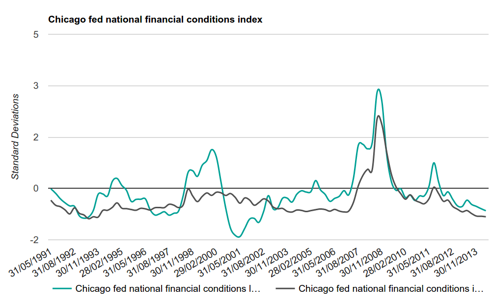
Fig. 8.1. NFCI
– ( margin debt ). .
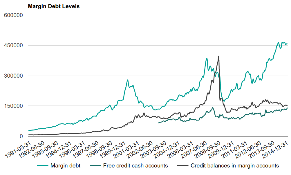
Fig. 8.2.
, . - . , . , . , , . , (Margin Call). , .
- , , , ? , , -, , , . , , , , , . ( deleveraging ).
, , , , . . 2008- 2009- S&P 500 30%, 8%.
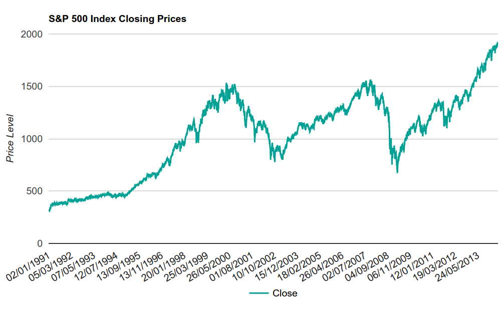
Fig. 9. S&P 500
, , , AIG, , . Lehman Brothers, , , , , , . , , , . , .
, , Lehman Brothers « » , , , , , . , Lehman Brothers, , , , . – . , , , , , . .
, . - , , 2010. , . , , , . , , 2012.
. . 2008- .
, , . , , - , – . So let's get started.
The financial crisis has swept around the world and significantly affected many people, including me. After I wrote this material, I sent it to friends and family. I wanted to express my own confidence that the duty of financial professionals is to remember that the road to hell is paved with good intentions, to remember that, just like in 2008, at any moment everything can go very easily So. And the first page from the Financial Times issue, which I mentioned at the beginning, hangs over my table as a reminder of the crisis.
Everything new is well forgotten old. Much has changed since the financial crisis of 2008. For example , the Volcker rule limited trading operations that banks could conduct, and the third part of the Basel Agreement and the Solvency II directive tightened capital requirements for banks, insurance companies and large hedge funds. The Dodd-Frank Act appeared , aimed at increasing responsibility and transparency in the financial system, at regulating bankruptcy procedures. However, much has remained the same since that time.
Governments are still making important economic decisions using outdated economic models. We are too much confident in the quantitative models, not understanding the assumptions underlying them. Margin trading connects the markets, seemingly having nothing in common, through the companies trading on them. Therefore, risk management is impossible without taking into account the correlation between markets and financial instruments.
I am sure that another financial crisis will happen in the end, although it will look different. I believe that some of the causes of the 2008 crisis, which I described, will still play a role in the economy. In addition, new operational risks are emerging. This is the growth of similar algorithmic trading systems, weakly connected electronic exchanges, and poorly designed software. All this has already shown its dark side in 1987 , and, most recently, during the instantaneous collapse of the stock market in 2010 . In my humble opinion, operational risks will play an increasingly important and dangerous role in the financial systems of the future.
The shock of meeting reality opened my eyes. The market is a complex adaptive system, within which are models and computer algorithms that almost no one understands. How can you not remember the words of Gordon Gekko from "Wall Street 2: Money does not sleep": "They call with different names multi-billion loans: CMO, CDO, SIV, MBS. I believe that only 75 people in the world know what it is. ”
Trying to understand and understand, I read books, studied programming, in the end I became the very “quant”, quantitative analyst, whose title did not cause anything but confusion before. Here is my vision of the financial crisis. I do not presume that my conclusions are the ultimate truth, but I rely on reliable data sources. My point of view was influenced by many books and articles read. Among them - “The big game for a fall”, “Quanta. Like math wizards, they earned billions and nearly collapsed the stock market, The Greatest Trade Ever, The Crisis of Crowding, Models Behaving Badly, and A Colossal Failure of Common Sense.
')
In fairness, it must be said that the financial crisis was caused not only by the collapse of credit derivatives. The cause of the crisis is a combination of many interrelated factors and problems. There are risks of bad faith, and illiterate economic policies, and deregulation of the financial sector. Excessive confidence of market participants in the used quantitative models, problems in insurance, too high level of use of borrowed funds on the stock exchange, availability of cheap money in the form of a loan and dangerous assumptions regarding market dynamics made a significant contribution to the development of the crisis. All of these factors, which I will discuss in more detail later, created a self-reinforcing model and led to a huge bubble in the market for credit derivatives. When it broke, the indirect connection of the markets, caused by the large leverage available on the stock exchange, led to a fall in the stock market.
I have divided the article into several sections, each of which gives a detailed account of why a particular factor caused the crisis. However, it is not necessary to read the sections sequentially. You may be returning from the next section to the previous section to assess the interdependence of factors. All the data I used to build graphs can be found on Quandl.com . In particular, from there I took information about interest rates and the real estate market in the USA. I used the data from Sifma.org to obtain data on credit derivatives issued, including credit default swaps (CDS) and debt collateral bonds (CDO).
Risks of bad faith
Risks of bad faith can occur in any situation where someone involved in a risky event knows that he is protected from loss, and someone else will cover the possible costs.
In my opinion, such a shift “from a sore head to a healthy one”, which occurred in mortgage lending, and led to a collapse. And this process itself, securitization, consists in transferring the risk from the lender to the investor by issuing securities that are secured by mortgage debt.
Mortgage banks issued to the borrowers a lump sum of money needed to buy a home in exchange for the borrower's obligation to repay the loan for 15-30 years, taking into account the appreciation rate (that is, with the interest of the bank).
There are two fundamentally different approaches to calculating the rate. The first is fixed. In this case, you can fix the amount of payments. The second is floating. With this approach, the loan rate may fluctuate over time. For example, if the bank believes that the risk of default or non-payment of a loan (say, you have delayed payment) increases, the bank may raise the rate. The same can happen if the central bank raises. That is, the higher the risk of default on the loan, the higher the rate on it. However, at that time everyone had a positive attitude, the rates were falling, so people more often took a mortgage with a floating rate, hoping for its decline in the future and not worrying that they can easily remain without work and cannot even at the minimum rate , pay the debt.
From the point of view of the creditor bank, the risk of default on a loan is on its balance sheet, so it has an incentive to issue as many mortgage loans as possible with the aim of earning more money in the future. From the point of view of the recipient of the loan, the interest on the loan is not as big as the prospect of an increase in the cost of housing that will pay back the interest rate. Except, of course, a situation where the lender is not knowingly going to repay the loan. This is the so-called strategic , planned default. Oliver Wyman conducted a study in 2009 and found that 20% of all defaults in 2008 were just that, and many of them were related to business lending.
Mortgage behaves in the same way as bonds, since the recipient of the mortgage is calculated on it every month, and, as a rule, does not allow default. The main difference between mortgages and bonds is that, as a rule, interest on mortgages is higher than on bonds, because housing prices, under the influence of rising demand, are growing rather quickly, and a loan, at least formally, is issued only to people with a good credit history. and rating, which reduces the likelihood of default on their part. At the same time, mortgage banks get a good profit.
The profits that mortgage banks received attracted the attention of experienced investors who invented the process of securitizing mortgage loans. This process allowed financiers to create a security whose payback was tied to monthly mortgage payments.
At first, the system worked quite well. If we explain this in a nutshell, the mortgage debt that was given to a particular borrower was transferred at a premium to the bank, which packed a lot of such loans into a security, and then sold it at a premium to investors under the guise of a reliable investment. And investors were happy to get a paper on which they received a coupon yield every month. Moreover, this approach has allowed mortgage banks to free up capital and issue more and more loans.
Such debt securities were given various names. For example, mortgage backed securities (MBS's), OBI - collateralized mortgage obligations (CMO's) and OBL - collateral debt obligations (CDO's). Some of these securities included not only mortgage debts of individuals, but also commercial mortgages, car loans, there was even credit card debt and much more. There are many subtleties associated with the process of securitization, which, unfortunately, are beyond the scope of this article. This is better to read on Wikipedia .
At first, the effect of the new debt securities was simply explosive. Turnover of mortgage banks has increased many times (this means that more people were able to buy houses), while banks resold debts to investors, who, in turn, received an investment instrument that brought more income than bonds at the same risk. However, with the spread of securitization, there was a problem, which was that the growth of new high-quality borrowers could not be infinite. It was here that the very risks of bad faith came into force - the mortgage borrower standard was falling.
Fig. 1. CDO market size in millions of US dollars
In order to meet the demand for new mortgage loans, lenders lowered standards of requirements for borrowers and began to lend to unreliable private clients, increasing the level of risk. New mortgage companies have entered the market. In particular, it has become popular to issue a floating rate mortgage to customers with a bad credit history and low reliability rating. Banks began issuing mortgages to several houses and low-income people at once. It all worked because the rates were artificially low, and housing prices were constantly rising. But as soon as that changed, the house of cards collapsed. People could no longer afford a monthly mortgage payment, an avalanche of defaults went. Purposeful defaults have also been added to them, since the cost of housing has fallen lower than the cost of the mortgage (often even without interest).
Fig. 2. The average price of homes sold
The above chart reflects the average selling price of a home in the United States, which is published quarterly. The graph shows that housing prices peaked at the end of 2006, and then began to fall, causing an increase in non-payments.
Fig. 3. Demand for new private homes
The above chart shows the demand for new private homes in the USA. Demand in 2006 began to fall. Most likely, this was the reason for the decline in real estate prices.
As already mentioned, artificially low interest rates set by the Fed contributed to the financial crisis. The reason for this was the previous crisis, which occurred when the dot-com bubble burst. Then the Fed lowered the rate to stimulate economic growth. Low rates remained for a very long time. This was a period when many mortgage borrowers took out a loan with a floating interest rate, because they believed that the rates would remain low always, which means that payments would be low. As a result, loans were taken even by those borrowers who could not afford them, and the banks, knowing that the client did not have the means to pay the mortgage, still issued loans, following the strategy of predatory lending .
Fig. 4. Floating lending rates
Interest rates represent debt service costs. When interest rates are low, debt service is cheap, and when interest rates are high, debts are expensive. The interest rate on the mortgage depends on the policy and interest rate of the Fed. So between 2004 and 2006, when the Federal Reserve increased interest rates, this led to an increase in mortgage rates. Many homeowners could no longer afford the monthly loan payments and began to purposefully declare defaults on the mortgage. This has not happened before.
Fig. 5. The share of loans with overdue payments
In each case of delay , the borrower has a certain period for repayment of the debt, then the lender can start a hearing on the rejection of the right to purchase housing and put it up for auction. This is what the average percentage of property alienations per 10,000 houses looks like according to data taken from here .
Fig. 6. The average percentage of property alienations for 10,000 homes
So, why did mortgage borrowers default? Here a combination of two factors worked. First, the average price of housing began to fall due to the fact that demand fell, and this spurred targeted defaults on mortgages, since the cost of housing was less than the cost of the loan. Secondly, the increase in mortgage rates put many borrowers in a difficult position, as they lost the ability to repay the loan and were forced to default.
However, the problems with loans alone could not cause a financial crisis. Next, we will discuss other factors that caused the crisis.
Modeling risks
In essence, all models are wrong, but some are useful. George Box
The use of quantitative models in finance has become almost ubiquitous, but it seems to me that very few of those who use these models understand the assumptions, initial assumptions, on which the models are built. “Modeling risk” is a term that I coined for this article, which means using a model to solve a problem without understanding the assumptions and limits of model applicability. In this section, I will discuss the use of a Gaussian copula to assess the correlation of credit defaults, and then make a small digression to talk about why machine learning today, in fact, is used incorrectly. Here you can read details about the sources of risk modeling.
Gaussian copula
Before we delve into the details of the Gaussian copula, the multidimensional distribution function, it is worth noting two fundamental postulates of modern portfolio theory. First, the unsystematic risk of the portfolio is less than or equal to the weighted sum of the unsystematic risks of each individual asset in the portfolio. Secondly, the level to which the unsystematic risk of a portfolio is reduced depends on the interdependence between the assets that make up the portfolio. In other words, by combining assets with a low level of correlation, we can build a portfolio that is less risky than individual assets. This approach is known as diversification.
Given this fact, and combining several credit derivatives, each of which is at risk of default, we will create a portfolio with a lower default risk than each of the tools individually. In other words, we can reduce the risk of credit default through diversification. At the turn of the millennium, the main question was how much diversification reduces risk. The answer to this question was a quantitative modeling method that demonstrated the correlation of possible defaults between independent credit derivatives.
Gaussian copula
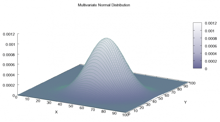
Gaussian copula is a multidimensional normal distribution. The figure shows a two-dimensional version.
In 2000, after the publication of the article “On Default Correlation: A Copula Function Approach”, David H. Lee was the first to use a Gaussian copula in modeling the correlation of defaults between credit derivatives in a portfolio. His work was inspired by how life insurance companies measure the risk of mortality or survival. In the annotation, Lee suggested that if the curve shows the probability of default of credit derivatives at any time before its maturity, then the probability that the portfolio of credit derivatives will default is determined by the joint distribution of the curves of each element of the portfolio. In actuarial mathematics, the most popular tools for calculating joint distribution are copulas. And the Gaussian copula is the most popular among them. Here is its formula:
Pr [T A <1, T B <1] = Φ 2 (Φ -1 (F A (1)), Φ -1 (F B (1)))
Here, Φ -1 (F A (1)) denotes the inverse function of the normal distribution function (quantile) of the cumulative distribution F A of the probability that credit derivative A will default next year. F A (1) and Pr [T A <1, T B <1] is a joint cumulative distribution function of the probability that credit derivatives A and B will default next year, and Φ 2 is a Gaussian copula. Such a copula usually shows that the probability of defaults of instruments A and B (correlation of defaults) is normally distributed. This assumption was probably made by using historical data that fit the model well, however, the problem is that the markets are changing.
There are two drawbacks with using a Gaussian copula, which lead to the fact that the model underestimates the risk of the credit derivatives portfolio. Underestimation of risk leads to an incorrect assessment of the value of derivatives, which, ultimately, has made a significant contribution to the financial crisis. The first drawback was in the calibration model, and the second - in the assumption of independence between the events of default on the loan. Ironically, both of these shortcomings (as well as some others), David H. Lee, drew attention in his article.
Calibration and stationarity
Lee suggested three possible model calibration methods:
- Use of historical data on defaults from rating agencies.
- Application of models based on the approach of Robert Merton.
- Apply an approach based on the use of market prices of bonds prone to default, or asset swap spreads.
In his material, Lee suggested using the third method. One of the reasons for this choice was, as he himself writes, the following: “Information that can be obtained from rating agencies usually include the probability of defaults by one year for each rating group and the rating migration matrix. Neither transition matrices nor default probabilities are necessarily stable [stationary] over long time intervals. In addition, the maturity of many credit derivatives significantly exceeds one year, which requires the use of a long-term marginal distribution of probabilities of defaults. ” This is exactly what we saw above. The probabilities of default, according to observations of historical information about default on obligations and data on property dispositions, are not stationary.
Since the model is calibrated according to historical data, according to rating agencies (which are also based on historical data), or at unreliable market prices, the model underestimates the risk of the credit derivatives portfolio. This was due to the fact that the historical distribution of the probability of defaults does not reflect the features of the future distribution. In other words, the distribution was and remains unsteady due to the fact that changing external factors, such as extremely low interest rates and risks of bad faith, radically changed the behavior of home buyers, thereby changing the likelihood of future credit defaults to the worse.
Risk independence assumption
Another problem with the model is that it allows for independence between the probabilities of credit default events in credit derivatives. Lee knew that such an assumption was dangerous and pointed out this: “the assumption of the independence of credit risks is obviously not realistic; in fact, the risk of default for a group of loans tends to increase during times of recession and to decrease in conditions of rapid growth of the economy. This implies that the same macroeconomic conditions affect each loan, and that there is some form of positive relationship between loans. ” This could be seen when the real estate market went down, and the number of defaults went up.
Despite the problems mentioned above, it is difficult to put the blame on what happened on David H. Lee and the Gaussian copula, since the copula is only a tool. Like any other tool, it has limitations. In the world of financial mathematics, these restrictions are now called model risk.
Model risk is the risk of loss caused by the use of a certain model when making decisions. After the financial crisis of 2008, much attention is paid to assessing the risk of using models in changing conditions. The market does not follow the rules, so nothing good from a blind faith in the model will not work.
Machine learning
Unfortunately, the same blind faith as in the case of quantitative models is now turned to machine learning models. New funds, making investment decisions, rely on neural networks. They do not care to understand the assumptions on which neural network models are built. For example, when building neural networks, it is assumed that the distribution of input patterns is stationary and does not contain outliers. The same is done when working with a Gaussian copula.
If the financial crisis taught us something, then this should be the understanding that the markets are constantly changing, and that there is nothing standard about them. I advocate the proper use of machine learning and quantitative models in the financial sector.
Insurance
In addition to credit derivatives whose value is tied to the underlying loans, banks and insurance companies have created derivatives that are tied to the level of defaults of these loans. These derivatives are called credit default swaps (CDS`s), they allow you to insure against default on debts, if defaults on loans underlying CDO lead to a decrease in the price of CDO. If you had such securities in 2007-2008, now you may have become rich and retired . 2008- 1000%.
CDS, .
, , , , . , , , 50%, 1000$. , 500$ 1000 . 500000$ (500$ * 1000), , , (1000$ * 1000 * 50%). , , , – 50$. $550000, – 500000$, 50000$.
, 50% ? , , , , 80% . 800000$, 250000$. , , .
, , , , 2008-. CDS, , , , , , . CDS, .
Fig. 7. CDS
, CDS, , . CDS AIG. , AIG , , . , AIG . AIG, , AIG.
– - . ( ) 1970- 2008- . .
: . 1929 – .
, 1990- , , , – , , .
, 2000- , – , , , (CDO) (CDS).
, , 2004- SEC , .
, , .
( national financial condition index , NFCI).
NFCI , , – . , (, ), .
Fig. 8.1. NFCI
– ( margin debt ). .
Fig. 8.2.
, . - . , . , . , , . , (Margin Call). , .
- , , , ? , , -, , , . , , , , , . ( deleveraging ).
, , , , . . 2008- 2009- S&P 500 30%, 8%.
Fig. 9. S&P 500
, , , AIG, , . Lehman Brothers, , , , , , . , , , . , .
, , Lehman Brothers « » , , , , , . , Lehman Brothers, , , , . – . , , , , , . .
, . - , , 2010. , . , , , . , , 2012.
. . 2008- .
, , . , , - , – . So let's get started.
- : .
- , 2000-.
- , (. 4).
- (. 4).
- , (. 3).
- , , (. 2).
- MBS, CDO .
- (AAA) . .
- , , (. 1).
- - (. 8).
- , .
- , , ( ).
- NINJA , .
- .
- (CDS). (. 7).
- AIG .
- 17 2004 2006- (. 4).
- , .
- , (. 2).
- . , (. 5 6).
- , .
- , , .
- (-) .
- , , , (. 8).
- , , - .
- , , AIG (. 9).
- Lehman Brothers .
- CDS , , AIG.
- AIG , .
- . .
- .
- , .
- 8% (. 9).
- ( TARP ). AIG.
- AIG , CDS, .
- , CDS. .
- 2008- 30% (. 9).
- , , , .
The financial crisis has swept around the world and significantly affected many people, including me. After I wrote this material, I sent it to friends and family. I wanted to express my own confidence that the duty of financial professionals is to remember that the road to hell is paved with good intentions, to remember that, just like in 2008, at any moment everything can go very easily So. And the first page from the Financial Times issue, which I mentioned at the beginning, hangs over my table as a reminder of the crisis.
Results
Everything new is well forgotten old. Much has changed since the financial crisis of 2008. For example , the Volcker rule limited trading operations that banks could conduct, and the third part of the Basel Agreement and the Solvency II directive tightened capital requirements for banks, insurance companies and large hedge funds. The Dodd-Frank Act appeared , aimed at increasing responsibility and transparency in the financial system, at regulating bankruptcy procedures. However, much has remained the same since that time.
Governments are still making important economic decisions using outdated economic models. We are too much confident in the quantitative models, not understanding the assumptions underlying them. Margin trading connects the markets, seemingly having nothing in common, through the companies trading on them. Therefore, risk management is impossible without taking into account the correlation between markets and financial instruments.
I am sure that another financial crisis will happen in the end, although it will look different. I believe that some of the causes of the 2008 crisis, which I described, will still play a role in the economy. In addition, new operational risks are emerging. This is the growth of similar algorithmic trading systems, weakly connected electronic exchanges, and poorly designed software. All this has already shown its dark side in 1987 , and, most recently, during the instantaneous collapse of the stock market in 2010 . In my humble opinion, operational risks will play an increasingly important and dangerous role in the financial systems of the future.
Source: https://habr.com/ru/post/398563/
All Articles