ATmega16 + DS18B20 + LED + Matlab / Simulink = AR
 I thought of somehow playing around with the DS18B20 sensors. And not just to get the temperature values (which everyone can do), but somehow to visualize it. There was a simple idea. We put a webcam. We light the light on an even frame, on an even one - simmer. Subtract the picture - only the flash remains. On it and look for the location of the sensor, which is physically attached to the LED in space. And then the mathematical processing. Well, all this in the simulator. Under the cut described how to get beautiful pictures. And for those who do not want to understand - I suggest to look at the experiments at the end of the article.
Circuitry
Circuitry is extremely simple. The heart is ATmega16. All DS18B20 sensors hang on the same pin (in my case on PB0 PORTB port). The pin itself is pulled to the supply voltage through a 4.7 kΩ resistor. The scheme is scalable. The picture is clickable.

All LEDs are connected to the PORTA port via limiting resistors. A gray polygon means that this LED is physically connected to the DS18B20. The reset pin is pulled to high through a 10 kΩ resistor to avoid accidental reset due to interference. The microcontroller is clocked with 16 MHz quartz. Put as close as possible to the conclusions. Loading capacities are used internal. Configured through fyuzy. Separately withdrawn connectors ICP (to fill the firmware) and UART for "communication". Capacities C1 (electrolyte 10 μF) and C2 (ceramics 100 nF). Put as close as possible to the power pins of the microcontroller. Used to avoid accidental drops during load transfer.
')
Circuitry assembly
What is a gray polygon
Firmware + work algorithm
The firmware was written in C in the Atmel Studio 7 IDE. Sources are posted on GitHub . The code is the most documented.
The project is divided into several levels of abstraction:
- Hardware - the lowest level, the maximum binding to the hardware. Work with the periphery of the microcontroller.
- Middleware - a link between Hardware and Drivers. For example, the implementation of the protocol 1-Wire.
- Drivers - driver level. For example, work with chip DS18B20.
- Application - the highest level of abstraction. For example, receiving and transmitting temperature via UART.
Run through the main function. First, there is a table of ROM addresses. It is necessary that the address of the sensor physically associated with the zero LED (hanging on the PA0 port of the PORTA) be in the zero position, and so on. For ROM, there is a function sendROMToUART . It is necessary only to remember that the sensor must be on the bus alone, otherwise there will be a collision of addresses.
main
int main(void) { const uint8_t ROM[][sizeof(ROM_T)] = /* ROM array */ { {0x26, 0x00, 0x00, 0x04, 0x4B, 0x15, 0x89, 0x28}, // 0 {0x71, 0x00, 0x00, 0x04, 0x4A, 0xC0, 0x65, 0x28}, // 1 {0xA5, 0x00, 0x00, 0x04, 0x4A, 0xCB, 0xCE, 0x28}, // 2 {0x41, 0x00, 0x00, 0x04, 0x4A, 0xAC, 0x65, 0x28}, // 3 {0x22, 0x00, 0x00, 0x04, 0x4B, 0x06, 0x0D, 0x28}, // 4 {0x86, 0x00, 0x00, 0x04, 0x4A, 0xF6, 0x46, 0x28} // 5 }; uint8_t nDevices = sizeof(ROM) / sizeof(ROM_T); /* Number of DS18B20 devices */ initUART(MYUBRR); /* Initialization of UART with appropriate baudrate */ initTimer0(); /* Initialization of Timer/counter0 */ initLED(nDevices); /* Initialization of LEDs */ { /* DS18B20s initialization */ uint8_t nDevices = sizeof(ROM) / sizeof(ROM_T); /* Number of DS18B20 devices */ ROM_T *pROM = (ROM_T *)&ROM; /* Pointer to ROM array */ initDQ(); /* Initialization of DQ pin */ while (nDevices--) /* For all DS18B20 */ initDS18B20(pROM++, RESOLUTION_11BIT); /* Initialization of DS18B20 with appropriate resolution */ } sei(); /* Global enable interrupts */ while (1) /* Infinite loop */ { sendTemperatureToUART((ROM_T *)&ROM, nDevices); /* Execute function routine */ } } Next is the initialization of the periphery and the DS-ok themselves with the appropriate resolution. The sampling period of the temperature depends on it. For 11 bits this is 375 ms. In an infinite loop, the program continuously reads the temperature from each sensor and sends it to the UART.
Work with LEDs is based on interruptions. The UART receives the ID of the LED 2 times in a row on an even and odd frame. At the first LED lights up. It extinguishes its timer after a certain time (in my case 15 ms). The second time just ignore. The timer is configured in CTC mode so that the interruption occurs every 1 ms.
code
volatile uint8_t ledID = 0; /* Current ledID value */ volatile uint8_t ledID_prev = 255; /* Previous ledID value */ volatile uint8_t duration = FLASH_DURATION; /* Flash duration value */ ISR(USART_RXC_vect) /* UART interrupt handler */ { ledID = UDR; /* Assign ledID to receive via UART value */ if (ledID != ledID_prev) /* If current ledID equal to previous value */ { turnOnLED(ledID); /* Turn on the ledID LED */ timer0Start(); /* Start Timer0 */ ledID_prev = ledID; /* Previous ledID assign to current */ duration = FLASH_DURATION; /* Update LED flash duration */ } } ISR(TIMER0_COMP_vect) /* Timer0 compare interrupt handler */ { if (--duration == 0) /* Decrement Duration value each 1ms and if it reach to 0 */ { timer0Stop(); /* Stop Timer0 */ turnOffAllLED(); /* Turn off all LEDs */ timer0Clear(); /* Clear Timer0 counter register */ } } The time sensitive parts of the code, which are 1-Wire signals, are wrapped in an ATOMIC_BLOCK construct. All basic settings are in global.h . The UART operates at a speed of 250000. Fast and error free for 16 MHz quartz. The driver DS18B20 has the functionality minimum necessary for this project. The rest - see the code. There will be questions - ask, do not hesitate. Separately, I want to remind you of the fusion settings. They need to set the clocking ability from external quartz otherwise it will be from the internal oscillator (and it is at most 8 MHz and not very stable). Well, program the CKOPT bit, otherwise quartz above 8 MHz will not start. I have High Fuse = 0xD9 , Low Fuse = 0xFF .
Simulink model + operation algorithm
Matlab R2015b version. In addition to the built-in library, Simulink mainly used Computer Vision System Toolbox and Image Aquisition Toolbox . The entire model and related files are uploaded to GitHub . Below is a detailed description with illustrative examples. All pictures are clickable.
WebCamTemp module
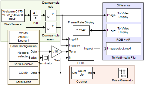 Blocks of a COM port are marked in yellow. Separately transmitter, receiver and configurator. Port settings must match exactly the microcontroller (speed, parity, number of bits, etc.). The receiver receives the temperature, grouping it into a one-dimensional array of size [n 1] of type int16 , where n is the number of DS18B20 (I have 6). Each element of this array is further divided by 16 . This is from datasheet page 6. The transmitter sends the current Counter value. It just lights a certain LED. Ticking from 0 to n . Period 2 sample. Blue are the blocks responsible for displaying / saving the video stream. Green - blocks receiving video. Actually the webcam itself. There are a lot of settings, different, depending on the manufacturer. The picture is issued in gray tones. That's more interesting. The Diff block makes the difference between the previous and current frames. The Downsample odd block highlights only the difference lit — not the lit LED, but not vice versa. The Downsample block even skips only those frames in which the LED is extinguished.
Img diff
On the left is the original, on the right is the difference picture. Further coordinates of the LEDs (respectively, of the sensors, too) are searched for. It is better to look at the frames, but apparently there is no such possibility in YouTube. You can set a speed of 0.25.
Img gray
On the left is the original, on the right is the picture on which the map is subsequently superimposed. After entering a stable mode, you can see that the LEDs do not blink. Made to not bothered.
Frame Rate Display displays the current FPS. All processing goes in the LEDs block. We will consider it as follows.
LEDs module
 Violet grouped blocks for obtaining 2D Gaussians . We need two: Interference and Opacity . Different sigma. Their center is at the maximum point (where the LED was on). The coordinates are located in the Maximum block. Instead of constantly generating such Gaussians (and the exponent is a very time-consuming mat. Operation), it was decided to cut them out. For this, in the m-file, two Int and Op are generated with dimensions 2 times larger with the center in the middle, of which, further, the necessary branches are simply sprinkled with Crop interference and Crop opacity blocks.
Work example
Top left is the input delta image. Bottom large - static image with a resolution twice as much as required. The running rectangle is the area that is cut with the desired resolution. At the top right - what we have at the exit. It is better to look at a speed of 0.25.
Green outlined memory blocks. Their purpose is to store the coordinates and gaussians for each LED. Take a closer look below. The To color block is designed for building temperature distribution and a color map. It will also be discussed below. Compositing signal composition block mixes two images Image1 and Image2 according to the following law:

The Insert Text block superimposes formatted text (in this case, temperature) on the image. Accepts n variables and coordinates in [XY] format. You can choose the font and its size. The blocks inside the red box implement the moving average algorithm . Transitions become less jerky, which saves nerves and pleases the eye.
Example
On the left is the original, on the right is the moving average for 8 samples. When the temperature of all sensors differ by a few tenths of degrees (a couple of sensor resolutions) such jerks take place.
Memory modules
Memory Interference and Memory opacity store 2D Gaussian sets, Memory Pts - coordinates for each LED.
Memory interference and Memory opacity These two modules are identical. At the input Address is the cell number where the input Gaussian is written. Comes from the counter. Coincides with the number of the burning LED. The Delay module of the LEDs module serves for additional synchronization (while the picture arrives, the counter has time to ottikat). So everything is synchronized. The Enable signal enables writing. It is true if the maximum value is above the threshold (see the Maximum and Threshold block of the LEDs module). If the value is false, the content of the cell does not change. At the exit, everything is glued together in the third dimension. It turns out such a sandwich size [HW n] , where HxW is the resolution of the webcam, and n is the number of sensors / LEDs.
These two modules are identical. At the input Address is the cell number where the input Gaussian is written. Comes from the counter. Coincides with the number of the burning LED. The Delay module of the LEDs module serves for additional synchronization (while the picture arrives, the counter has time to ottikat). So everything is synchronized. The Enable signal enables writing. It is true if the maximum value is above the threshold (see the Maximum and Threshold block of the LEDs module). If the value is false, the content of the cell does not change. At the exit, everything is glued together in the third dimension. It turns out such a sandwich size [HW n] , where HxW is the resolution of the webcam, and n is the number of sensors / LEDs.Memory Pts Identical to the previous two, with a few exceptions. At the exit, everything is glued together not in the third but in the first dimension. And the Permute Matrix block simply swaps the columns, since the coordinate format is [YX] , but [XY] is needed.
Identical to the previous two, with a few exceptions. At the exit, everything is glued together not in the third but in the first dimension. And the Permute Matrix block simply swaps the columns, since the coordinate format is [YX] , but [XY] is needed.To color module
 Green is Opacity processing. We summarize the input array in the third dimension. Normalize it to the maximum. Multiply by the value of gain (from 0 to 1) (1) . Total we have an array with Gaussians superimposed on each other and maximum gain . Used as a factor for image blending. Red — Get a color temperature map. There is a slightly different math, all the same Gaussians. Described by the formula (2) . Roughly speaking, the temperature at an arbitrary point is the weighted average of all sensors. But the influence of each sensor as a percentage is proportional to the value of the Gaussians in it. The sum of all is taken as 100%.
 It remains to consider how the temperature distribution turns into a color map. The fact that circled in blue turns the specific temperature into a value between 0 and 1. In the red zone, the Prelookup block calculates the index by which the red, green, and blue value is searched. An array of colors contains 64 values. Intermediate are calculated by interpolation. Of the features there are two modes: relative and absolute. In the relative coldest and hottest place corresponds to the minimum and maximum of the input array. In the absolute - some constant values. In the first, it is more convenient to look at the temperature distribution profile. In the other - her absolute changes.
m-file
It is executed at the beginning, before the simulation, introducing variables into the Workspace.
code
H = 480; % Height of image W = 640; % Width of image minT = 20; % Min temperature maxT = 25; % Max temperature sigmaInt = 40; % Sigma interference sigmaOp = 80; % Sigma opacity gain = 1.0; % Gain value T = 0.3; % Threshold value nAvr = 8; % number of means % ------------------------------------------------------ [M,N] = meshgrid(-W:W, -H:H); % Meshgrid function R = sqrt(M.^2 + N.^2); % Distance from the center Int = normpdf(R, 0, sigmaInt); % 2D gaussian for interference Op = normpdf(R, 0, sigmaOp); % 2D gaussian for opacity Int = Int/max(max(Int)); % Normalization of interference gaussian Op = Op/max(max(Op)); % Normalization of opacity gaussian clear MNR sigmaInt sigmaOp % Delete unused variables from memory load('MyColormaps','mycmap'); % Load colormap It contains the main control variables including:
- H - video resolution in height.
- W - video resolution in width.
- minT is the minimum absolute temperature.
- maxT is the maximum absolute temperature.
- sigmaInt - Sigma Gaussian Interference.
- sigmaOp - sigma gaussians Opacity.
- gain is the maximum factor value.
- T - threshold to avoid errors.
- nAvr is the number of averages for the moving average.
H and W must match the current one in the WebCamera block. minT and maxT affect the color map in absolute temperature mode. T is set from 0 to 1. Sometimes the COM port and the webcam are out of sync. The phase of the differential image can change by 180 °. And where there should be a maximum - there is a minimum. And the coordinate system can choose arbitrary - not corresponding to reality. For this, there is a threshold system. nAvr number of averages on a moving average. The larger it is, the smoother the transitions, but relevance is lost (a time shift appears). To understand the influence of the remaining variables, no clear examples can not figure out.
SigmaInt effect
With  the picture degenerates into some sort of Voronoi partition . With
  the whole map will be of the same color as the average, from all sensors, temperature. With an increase - the boundaries are blurred.
the picture degenerates into some sort of Voronoi partition . With the whole map will be of the same color as the average, from all sensors, temperature. With an increase - the boundaries are blurred.SigmaOp effect
Sets the decay rate of transparency from a distance.
Effect of gain
Essentially sets the transparency of the map. The value itself corresponds to the “transparency” of the most “non-transparent” pixel of the map.
Experiments
Below are some experiments.
Open window
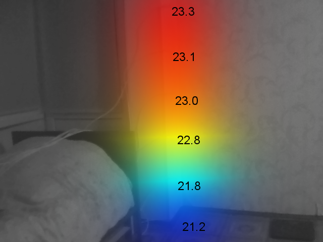
Sensors are scattered on the bed by the window. The window opens and closes after a while. A vivid example of the difference in relative (left) and absolute (right) modes. With the help of the first, it is convenient to consider the distribution, and the second - how the cold spreads or the heat recovers.
Window sill
Sensors are located along the window sill. The window opens - the profile is changing. The coldest and warmest zones are clearly visible.
Top warmer?
They say the pier is warmer on top. This experiment is a complete confirmation of this. On the 10th second the window opens, on the 30th second it closes.
Conclusion
Such a scheme will not replace a full-fledged thermal imager. But he is not able to see the spread of air masses. And at the price this design is incommensurably lower. You can use a different color map. You can take other functions instead of Gaussians. You can even change the laws of construction. Or rewrite to OpenCV + QT for speed and convenience. But that which I planned was achieved. Just Just For Fun .
Source: https://habr.com/ru/post/390985/
All Articles