The first Soviet AVM
In 1945 - 1946 under the leadership of L.I. Gutenmahera developed the first electronic analog machines with a repetition of the solution. But since 1949, a team of Soviet developers headed by VB. Ushakov and V.A. Trapeznikov, invented a number of AVM on direct current. This year began the history of the development of analog computing in the USSR. The use of operational amplifiers, which worked on the principle of automatic control systems with deep negative feedback, made it possible to carry out accurate modeling of mathematical operators, as well as parallel processing of information in real time when solving systems of differential equations.
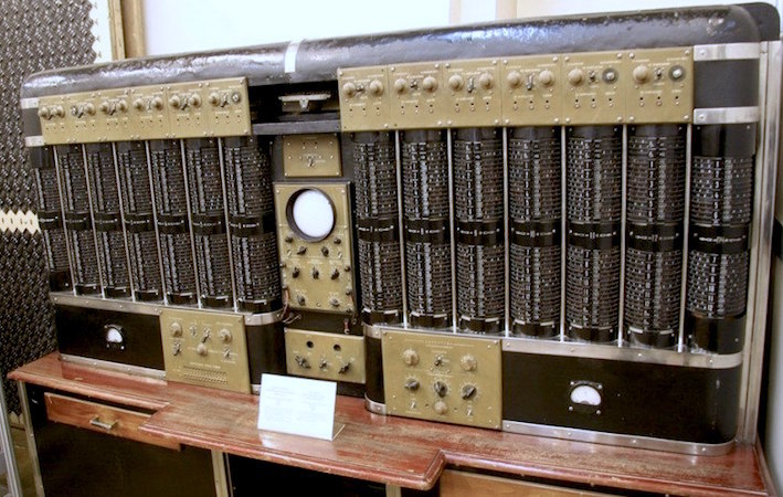
In 1949, the laboratory of electrical ITMiVT and department of the chief designer of the Penza plant SAM BA. Matkina was released electron-tube integrator ELI-12. It was intended for solving a system of 12-order differential equations with constant coefficients and constant right-hand sides. The process of solving the problem was automatically repeated, in consequence of which the results of the solution were displayed, measured and photographed on the CRT screen.
')

After finalizing the circuits and design of the electron-tube integrator, as well as preparing for industrial production, the factory began mass production of ELI-12-1.
The integrator ELI-14 was developed on its schematic design basis, where differential equations of the sixth order were solved. There were 6 decision blocks. For the manufacture of switching tubes used neolikorite, which is characterized by high insulating properties.
In 1949–1950 in NII-885 team led by VB Ushakov created the first AVMs, which were called DC integrators. In 1949 - IPT-1, IPT-2 and IPT-3; in 1950, IPT-4 and IPT-5, which are mass-produced. These machines were designed to solve linear differential equations with constant and variable coefficients. Thanks to operational amplifiers, AVM provided solutions to the most important tasks in various scientific and technical fields (aviation, rocket production, space research, defense industry, etc.).
The first AVMs on electron tubes were created by the joint efforts of two teams: NII-855 MRP USSR and IAT of the Academy of Sciences of the USSR. The serial production of AVM was organized at the Moscow, Penza and Kishinev factories of calculating-analytical machines and a number of other plants of the radio industry.
Developed in 1952-1953. under the leadership of V. B. Ushakov, AVM received the name "DC Simulation Units" (MPT). Serial AVM "MPT-9" were intended to solve linear differential equations, "MPT-11" - to solve nonlinear differential equations.
In 1955 the first Soviet precision high-power AVM MN-8 was developed. She was the largest non-linear electronic mathematical machine of continuous action. The development team was headed by VB Ushakov. The machine should solve the sixteenth and higher order differential equations (32 integrating units). In the case of the sixteenth order, half the linear part was used.

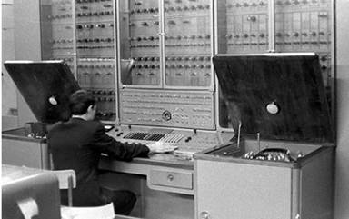
The electronic simulation installation consisted of 13 sections. Tasks were gathered using cord connections on the switching fields of the linear part. By means of a pair of control panels, two different tasks were simultaneously solved. The maximum duration of the integration process reached 10,000 seconds, and the power consumption was 25 kW.
MN-8 carried out up to 48 summation operations, 264 terms, 48 multiplications per constant coefficient, 36 multiplications per variable coefficient, 12 exact multiplications of the unknown quantities. There was also the possibility of a set of 10 non-linear dependencies of a function on one variable, 40 non-linear dependencies of the signature type, 9 non-linear dependencies of typical characteristics (backlash, restrictions, dead zones).
In the car, there were 400 operational amplifiers with individual automatic zero stabilization and an improved circuit for their control. Through powerful amplifiers with an economical output, interaction with real equipment took place. The control circuit had additional control.
Only three foreign models could compare with the Soviet model:
- American electrical installation "Typhoon" (Typhoon), released in 1951;
- English electrical installation "Tridak" ("Trydac" - Three Dimensional Analogue Computer), was created in the period 1950-1954. She was an electronic-hydraulic simulator, with which shells control was investigated;
- American installation “Convair” (“Convair”), released in 1954
The peculiarity of “MN-8” was that the duration of the processes studied by the installation on a natural time scale could be both small (a few seconds) and very significant.
The scheme of the integrating unit accelerated the expansion process, it allowed to automatically change the time scale simultaneously for all such installation units 10 times.

In MN-8, precision multiplication units were used. They made it possible to obtain the static accuracy of the multiplication operation about ± 0.01%. The number of blocks in the machine made it possible to obtain 12 operations of exact multiplication of variables.
The MN-8 consisted of 48 precise blocks for inputting variable coefficients, which practically reproduced the graph of the variable coefficient using the piecewise linear approximation method. And also included 40 special non-linear blocks to perform non-linear dependencies of the signature type. This improvement has greatly expanded the capabilities of the machine.
The Soviet electrical plant had an improved control circuit. On the basis of a decimal digital counter, an electronic block of a time meter was built. It was used to synchronize the work of all functional units. The decision process could be periodically repeated or stopped at predetermined time intervals.
In MN-8, diode-triode electronic circuits were used for universal units, which were intended to reproduce nonlinear functions of one variable with the accuracy of the set of functions ± 0.2.
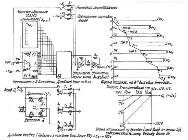
The block allowed to gain very steep fronts of the function, as well as functions with sharp kinks.
The simulated system of equations was typed in accordance with the block diagram of the solution of the problem on the switching fields that were on sections of the linear units of the installation. Trunk lines between sections made it possible to use blocks of neighboring sections in one task. In "MN-8" there were no removable switching fields.
Registration and control of output values were carried out with the help of six high-speed electronic potentiometers, an electronic-digital voltmeter, an electron-beam indicator and other measuring devices.
The "MN-8" there were 14 racks. The design of the device used small blocks, so that it was relatively compact. The circuit of the electrical installation consisted of many high-quality electrical components (they significantly increased the accuracy of work). For example, about 8,000 germanium plane diodes were used in the power section circuitry.
The MN-8 was mass-produced by the Penza CAM plant.
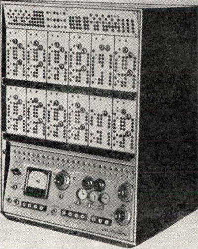
In 1958, the electronic modeling installation "MN-9". It was intended to study the dynamics of the main parts of the clock mechanism. The development was led by chief designer I.M. Vitenberg.
The "MN-9" was a bench design. With the help of switches and knobs, placed on the front panels of the machine, installed modes of work.
"MN-9" solved systems of ordinary linear equations with variable coefficients. The device consisted of 5 blocks of summing amplifier, 40 blocks of constant coefficients and 9 blocks of non-linear function of one variable. The “MN-9” had 28 amplifiers with centralized automatic setting of zeros according to a circuit with capacitors and is characterized by the presence of an electronic circuit for automatic switching of the machine’s units as a function of the desired variable.
The electronic modeling installation "MN-9" was not produced commercially.
In 1957, a new development of Soviet specialists came out - a small-sized non-linear tubeless modeling installation "MN-10". It was the first analog computing machine with a circuit completely made on semiconductor elements. With the help of the installation, problems that were described by ordinary nonlinear differential equations were solved and investigated. For example, this:

where i = 1, 2, ..., 6.
Including the installation made it possible to solve differential equations, which contained up to 6 non-linear dependencies of the type of function on one variable or the product of two variables. Work could be carried out on a natural time scale. The results of the tasks were demonstrated on an electron-beam indicator such as I-5 or I-4.
The “MN-10” consisted of 24 small-sized operational DC amplifiers. They performed the operations of integration, differentiation, summation and large-scale transformations. There are also 4 diode cells, which were used in schemes that reproduce typical nonlinear dependences of the type of hysteresis loop, dry friction torque, deadband, and constraints.
The device occupied an area of 0.3 m 2 , weighed 75 kg. The range of change of variables of the installation ranged from 30 V to +30 V. The duration of the integration process was 200 seconds.
Food "MN-10" came from the unit ESV-10, included in its kit. And the power from the network was supplied by a single-phase alternating current of 220 V, frequency 50 Hz. The power consumption was 100 watts.
In the 70s, the installation was upgraded and began to be mass-produced.
Analog computer "MN-10M" was developed by experts of the Penza plant. The model belonged to small-sized desktop machines of low power, with the help of which real dynamic systems were investigated by the method of mathematical modeling. Also "MN-10M" was intended to integrate ordinary differential equations of no higher than tenth order.
Machine dimensions were 460 × 615 × 445 mm., And weight - 50 kg. The "MN-10M" consisted of 24 operational amplifiers, as well as a set of 12 feedbacks.
Thanks to a set of operating units, it was possible to perform various operations:
- integration operations with simultaneous summation (up to 10);
- operations of inversion or summation (up to 24);
- setting on voltage dividers (up to 60 constant coefficients);
- reproduction of unambiguous continuous nonlinear functions of one variable with simultaneous summation of several variables;
- the operation of multiplication or division with the simultaneous summation of several variables;
- reproduction of up to 6 typical non-linear dependencies of the type of dead zone, limitation, dry friction;
- operations of conditional transition (up to 4).
More complex problems were solved in parallel by two or three MN-10M machines. It was possible to observe and measure the result of the task using a switch instrument of the machine or an external recording device (DRP, EPP-09, loop-oscillograph). They were not part of the car.
Provided mate with external equipment. Food "MN-10M" came from the ESW-4 unit, which was included in its kit. And the power from the network was supplied by a single-phase alternating current of 220 V, frequency 50 Hz. The power consumption was 250 watts. The circuit of the machine and power supply was completely built on semiconductor elements.
The machine solved ordinary differential equations. The range of change of variables was from - 25 V to + 25 V. The duration of the integration process was 200 seconds.
The MN-10M unit included an electronic stabilized rectifier (ESV-4), an analog computer of communication (AVM), communication channels with external equipment, with the second and with the third machine.
More than 100,000 AVMs were manufactured in the first 20 years. From simple to the most powerful, like "MN-8". At first, the machines were used mostly as independent tools for mathematical modeling of dynamic objects in real time. But approximately in the 1960s and 1970s, progress in the field of digital electronics required the joint processing of AVM and DVM information.
Start of development
In 1949, the laboratory of electrical ITMiVT and department of the chief designer of the Penza plant SAM BA. Matkina was released electron-tube integrator ELI-12. It was intended for solving a system of 12-order differential equations with constant coefficients and constant right-hand sides. The process of solving the problem was automatically repeated, in consequence of which the results of the solution were displayed, measured and photographed on the CRT screen.
')
After finalizing the circuits and design of the electron-tube integrator, as well as preparing for industrial production, the factory began mass production of ELI-12-1.
The integrator ELI-14 was developed on its schematic design basis, where differential equations of the sixth order were solved. There were 6 decision blocks. For the manufacture of switching tubes used neolikorite, which is characterized by high insulating properties.
In 1949–1950 in NII-885 team led by VB Ushakov created the first AVMs, which were called DC integrators. In 1949 - IPT-1, IPT-2 and IPT-3; in 1950, IPT-4 and IPT-5, which are mass-produced. These machines were designed to solve linear differential equations with constant and variable coefficients. Thanks to operational amplifiers, AVM provided solutions to the most important tasks in various scientific and technical fields (aviation, rocket production, space research, defense industry, etc.).
The first AVMs on electron tubes were created by the joint efforts of two teams: NII-855 MRP USSR and IAT of the Academy of Sciences of the USSR. The serial production of AVM was organized at the Moscow, Penza and Kishinev factories of calculating-analytical machines and a number of other plants of the radio industry.
Developed in 1952-1953. under the leadership of V. B. Ushakov, AVM received the name "DC Simulation Units" (MPT). Serial AVM "MPT-9" were intended to solve linear differential equations, "MPT-11" - to solve nonlinear differential equations.
"MN-8"
In 1955 the first Soviet precision high-power AVM MN-8 was developed. She was the largest non-linear electronic mathematical machine of continuous action. The development team was headed by VB Ushakov. The machine should solve the sixteenth and higher order differential equations (32 integrating units). In the case of the sixteenth order, half the linear part was used.
The electronic simulation installation consisted of 13 sections. Tasks were gathered using cord connections on the switching fields of the linear part. By means of a pair of control panels, two different tasks were simultaneously solved. The maximum duration of the integration process reached 10,000 seconds, and the power consumption was 25 kW.
MN-8 carried out up to 48 summation operations, 264 terms, 48 multiplications per constant coefficient, 36 multiplications per variable coefficient, 12 exact multiplications of the unknown quantities. There was also the possibility of a set of 10 non-linear dependencies of a function on one variable, 40 non-linear dependencies of the signature type, 9 non-linear dependencies of typical characteristics (backlash, restrictions, dead zones).
In the car, there were 400 operational amplifiers with individual automatic zero stabilization and an improved circuit for their control. Through powerful amplifiers with an economical output, interaction with real equipment took place. The control circuit had additional control.
Only three foreign models could compare with the Soviet model:
- American electrical installation "Typhoon" (Typhoon), released in 1951;
- English electrical installation "Tridak" ("Trydac" - Three Dimensional Analogue Computer), was created in the period 1950-1954. She was an electronic-hydraulic simulator, with which shells control was investigated;
- American installation “Convair” (“Convair”), released in 1954
The peculiarity of “MN-8” was that the duration of the processes studied by the installation on a natural time scale could be both small (a few seconds) and very significant.
The scheme of the integrating unit accelerated the expansion process, it allowed to automatically change the time scale simultaneously for all such installation units 10 times.
In MN-8, precision multiplication units were used. They made it possible to obtain the static accuracy of the multiplication operation about ± 0.01%. The number of blocks in the machine made it possible to obtain 12 operations of exact multiplication of variables.
The MN-8 consisted of 48 precise blocks for inputting variable coefficients, which practically reproduced the graph of the variable coefficient using the piecewise linear approximation method. And also included 40 special non-linear blocks to perform non-linear dependencies of the signature type. This improvement has greatly expanded the capabilities of the machine.
The Soviet electrical plant had an improved control circuit. On the basis of a decimal digital counter, an electronic block of a time meter was built. It was used to synchronize the work of all functional units. The decision process could be periodically repeated or stopped at predetermined time intervals.
In MN-8, diode-triode electronic circuits were used for universal units, which were intended to reproduce nonlinear functions of one variable with the accuracy of the set of functions ± 0.2.
The block allowed to gain very steep fronts of the function, as well as functions with sharp kinks.
The simulated system of equations was typed in accordance with the block diagram of the solution of the problem on the switching fields that were on sections of the linear units of the installation. Trunk lines between sections made it possible to use blocks of neighboring sections in one task. In "MN-8" there were no removable switching fields.
Registration and control of output values were carried out with the help of six high-speed electronic potentiometers, an electronic-digital voltmeter, an electron-beam indicator and other measuring devices.
The "MN-8" there were 14 racks. The design of the device used small blocks, so that it was relatively compact. The circuit of the electrical installation consisted of many high-quality electrical components (they significantly increased the accuracy of work). For example, about 8,000 germanium plane diodes were used in the power section circuitry.
The MN-8 was mass-produced by the Penza CAM plant.
"MN-9"
In 1958, the electronic modeling installation "MN-9". It was intended to study the dynamics of the main parts of the clock mechanism. The development was led by chief designer I.M. Vitenberg.
The "MN-9" was a bench design. With the help of switches and knobs, placed on the front panels of the machine, installed modes of work.
"MN-9" solved systems of ordinary linear equations with variable coefficients. The device consisted of 5 blocks of summing amplifier, 40 blocks of constant coefficients and 9 blocks of non-linear function of one variable. The “MN-9” had 28 amplifiers with centralized automatic setting of zeros according to a circuit with capacitors and is characterized by the presence of an electronic circuit for automatic switching of the machine’s units as a function of the desired variable.
The electronic modeling installation "MN-9" was not produced commercially.
"MN-10"
In 1957, a new development of Soviet specialists came out - a small-sized non-linear tubeless modeling installation "MN-10". It was the first analog computing machine with a circuit completely made on semiconductor elements. With the help of the installation, problems that were described by ordinary nonlinear differential equations were solved and investigated. For example, this:
where i = 1, 2, ..., 6.
Including the installation made it possible to solve differential equations, which contained up to 6 non-linear dependencies of the type of function on one variable or the product of two variables. Work could be carried out on a natural time scale. The results of the tasks were demonstrated on an electron-beam indicator such as I-5 or I-4.
The “MN-10” consisted of 24 small-sized operational DC amplifiers. They performed the operations of integration, differentiation, summation and large-scale transformations. There are also 4 diode cells, which were used in schemes that reproduce typical nonlinear dependences of the type of hysteresis loop, dry friction torque, deadband, and constraints.
The device occupied an area of 0.3 m 2 , weighed 75 kg. The range of change of variables of the installation ranged from 30 V to +30 V. The duration of the integration process was 200 seconds.
Food "MN-10" came from the unit ESV-10, included in its kit. And the power from the network was supplied by a single-phase alternating current of 220 V, frequency 50 Hz. The power consumption was 100 watts.
In the 70s, the installation was upgraded and began to be mass-produced.
"MN-10M"
Analog computer "MN-10M" was developed by experts of the Penza plant. The model belonged to small-sized desktop machines of low power, with the help of which real dynamic systems were investigated by the method of mathematical modeling. Also "MN-10M" was intended to integrate ordinary differential equations of no higher than tenth order.
Machine dimensions were 460 × 615 × 445 mm., And weight - 50 kg. The "MN-10M" consisted of 24 operational amplifiers, as well as a set of 12 feedbacks.
Thanks to a set of operating units, it was possible to perform various operations:
- integration operations with simultaneous summation (up to 10);
- operations of inversion or summation (up to 24);
- setting on voltage dividers (up to 60 constant coefficients);
- reproduction of unambiguous continuous nonlinear functions of one variable with simultaneous summation of several variables;
- the operation of multiplication or division with the simultaneous summation of several variables;
- reproduction of up to 6 typical non-linear dependencies of the type of dead zone, limitation, dry friction;
- operations of conditional transition (up to 4).
More complex problems were solved in parallel by two or three MN-10M machines. It was possible to observe and measure the result of the task using a switch instrument of the machine or an external recording device (DRP, EPP-09, loop-oscillograph). They were not part of the car.
Provided mate with external equipment. Food "MN-10M" came from the ESW-4 unit, which was included in its kit. And the power from the network was supplied by a single-phase alternating current of 220 V, frequency 50 Hz. The power consumption was 250 watts. The circuit of the machine and power supply was completely built on semiconductor elements.
The machine solved ordinary differential equations. The range of change of variables was from - 25 V to + 25 V. The duration of the integration process was 200 seconds.
The MN-10M unit included an electronic stabilized rectifier (ESV-4), an analog computer of communication (AVM), communication channels with external equipment, with the second and with the third machine.
More than 100,000 AVMs were manufactured in the first 20 years. From simple to the most powerful, like "MN-8". At first, the machines were used mostly as independent tools for mathematical modeling of dynamic objects in real time. But approximately in the 1960s and 1970s, progress in the field of digital electronics required the joint processing of AVM and DVM information.
Source: https://habr.com/ru/post/390599/
All Articles