Kinematics delta robot

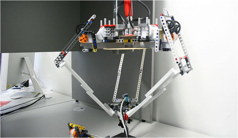
Back in 2009, I got excited about the idea of building my own industrial robot that could do something useful (namely, sort small parts on the conveyor). I’ll say right away that I built a robot (you see the result in the title photo), and at the same time, as a by-product, I wrote a short article about the kinematics of delta robots on the TrossenRobotics forum - an American seller of sets of parts for robots. At that time they were holding a contest for authors. Of course, I did not win the contest, but the article in English remained. Several times I tried to translate it into my native language, but I managed to complete the job just now.

If you want to build your own model of a delta robot, or just figure out how to derive kinematic formulas for this type of robot (without going beyond the school program in algebra and geometry) - welcome to cat. For those who are not very fond of theory, at the end of the article are examples of ready-made code in C.

What is a delta robot

Delta-robot ( wiki ) was invented in the early 1980s by the Swiss scientist Raymond Clavel, below is an illustration from the original patent US4976582 on "A device for moving and positioning an element in space":
')

The robot consists of two platforms: a fixed upper base (1) and a small mobile platform (8), connected by three levers. Each lever consists of two parts: the upper arm (4) is rigidly connected to the engine (3) located on the upper base, and the lower arm is a parallelogram (5), in the corners of which are installed the so-called. universal joints (6, 7) ( wiki ) that allow angles to change. Each parallelogram is connected to the upper arm by the hinge (16) so that its upper side always remains perpendicular to its lever and parallel to the plane of the upper base. Due to this, the mobile robot platform attached to the lower sides of the parallelograms will also always be parallel to the upper base. We can control the position of the platform by changing the angle of rotation of the upper arms relative to the base of the robot with the help of engines.

In the center of the lower platform (8) is attached the so-called. the working body (in English they use the term end effector) of the robot (9). This may be a manipulator, a gripping device or, for example, an extruder in the case of a 3D printer. Additionally, another engine (11) can be used, which provides rotation of the working element through the rod (14).

The main advantage of delta robots is speed: heavy engines are placed on a fixed base, only levers and a lower platform move, which they try to make from light composite materials, thereby reducing their inertia. Here, for example, article on Geektimes with a couple of very spectacular videos.

Task statement

To build your own delta robot, you need to learn how to solve two problems. In the first situation, we know the position to which we want to move the robot's manipulator (for example, we want to grab a cookie that is on a conveyor at a point with coordinates (x, y, z) . To do this, we need to determine the angles to which we They must turn the engines connected with the levers of the robot to set it in the correct position to grip.The procedure for determining these angles is called the inverse (in some Russian-language sources the word “inverse” is used) kinematic task.
In the second situation, we know the angles that the robot control motors are turned on (if we use servomotors, then the angles can be easily recognized by reading the readings from the angle sensors), and we want to find the position of the robot platform in space (for example, to correct its position) . This is a direct kinematic problem.

We formalize both problems. Both the motionless base of the robot and its moving platform can be represented as equilateral triangles: in the diagram below, they are painted in green and pink, respectively. The rotation angles of the levers of the robot relative to the plane of the base (they are also the angles of rotation of the motors) are designated as Ѳ ₁ , ₂ and Ѳ ₃ , and the coordinates of the E ₀ point located in the center of the mobile platform and in which the robot arm will be fixed in real life (x ₀ , y ₀ , z ₀ ) .

It turns out that we have to come up with two functions:

f _inverse (x ₀ , y ₀ , z ₀ ) → (Ѳ ₁ , Ѳ ₂ , Ѳ ₃ ) to solve the inverse kinematic problem and
f _forward (Ѳ ₁ , Ѳ ₂ , ₃ ) → (x ₀ , y ₀ , z ₀ ) to solve the direct kinematic problem.

Inverse kinematics

Let's set some key parameters which are defined by the geometrical sizes of our robot:

Denote the length of the side of the upper base f , the side of the lower platform e , the length of the upper arm of the lever r _f and the length of the lower arm (the long side of the parallelogram) r _e . For calculations, we choose a coordinate system with a reference point that coincides with the geometric center of the upper triangle. We will direct the Z axis upwards, so the z-coordinate of the mobile platform will always be negative.

The design of the robot implies that the lever F ₁ J ₁ (see figure below) can only rotate in the YZ plane, describing a circle with a radius of r _f centered at the point F ₁ (in this place it is attached to the engine). Unlike F ₁ , nodes J ₁ and E ₁ use universal joints, due to which arm E ₁ J ₁ can freely rotate relative to E ₁ , describing a sphere of radius r _e centered at point E ₁ .

The intersection of this sphere and the YZ plane is a circle centered at the point E ' _{1 with a} radius E' ₁ J ₁ , where the point E ' ₁ lies as the projection of the point E ₁ onto the YZ plane. Then the point J ₁ will be located at the intersection of two circles with centers at the points E ' ₁ and F ₁ , and we can determine the radii of these circles. There is a small subtlety: the circles intersect at two points, but we are only interested in one of them - with a smaller value of the y coordinate, since we want the levers of the robot to always stick out "elbows" outwards. Having thus determined the coordinates of the point J ₁ , we can easily find the angle of interest to us ₁ .

For convenience, the projection of our three-dimensional image on the YZ plane is shown below:

The lower platform is an equilateral triangle whose center is the point E ₀ (x ₀ , y ₀ , z ₀ ) . Mean distance

$E_0E_1 = {e \ over2} \ tan (30 ^ o) = {e \ over2 \ sqrt3},$

which gives us the following coordinates of the point E ₁ and its projection E ' ₁ on the YZ plane:

$E_1 (x_0, y_0- {e \ over2 \ sqrt3}, z_0) \ Rightarrow E'_1 (0, y_0- {e \ over2 \ sqrt3}, z_0)$

The distance E ₁ E ' ₁ = x ₀ , then, according to the Pythagorean theorem,

$E'_1J_1 = \ sqrt {E_1J_1 ^ 2-E_1E'_1 ^ 2} = \ sqrt {r_e ^ 2-x_0 ^ 2}$

Since the upper platform is also an equilateral triangle, the coordinates of the point F ₁ will be

$F_1 (0, {-f \ over {2 \ sqrt3}}, 0)$

To find the coordinates of the point J ₁ , which is the intersection of two circles, it is necessary to solve the system of equations:

$\ begin {equation *} \ begin {cases} (y_ {J_1} -y_ {F_1}) ^ 2+ (z_ {J_1} -z_ {F_1}) ^ 2 = r_f ^ 2 \\ (y_ {J_1} - y_ {E'_1}) ^ 2+ (z_ {J_1} -z_ {E'_1}) ^ 2 = r_e ^ 2-x_0 \ end {cases} \ end {equation *}$

The coordinates of the centers of the circles are known to us; if we substitute them, we get the following expression:

$\ begin {equation *} \ begin {cases} (y_ {J_1} + {f \ over {2 \ sqrt3}}) ^ 2 + z_ {J_1} ^ 2 = r_f ^ 2 \\ (y_ {J_1} -y_0 + {e \ over {2 \ sqrt3}}) ^ 2+ (z_ {J_1} -z_0) ^ 2 = r_e ^ 2-x_0 \ end {cases} \ end {equation *}$

If we expand the brackets and subtract one equation from another, we can express the z-coordinate of the point J ₁ in a linear way through the y-coordinate, then, substituting it into the second equation, we get the usual quadratic equation for y, from the two solutions of which we choose the smallest we spoke above). And having thus obtained the coordinates of the point J ₁ , we find the angle

$\ theta_1 = \ arctan \ left ({z_ {J_1} \ over {y_ {F_1} -y_ {J_1}}} \ right)$

All the expressions turned out to be quite simple due to the successful choice of the coordinate system: the lever arm F ₁ J ₁ always moves in the YZ plane, so we can simply ignore the x coordinate. To maintain this advantage when finding the two remaining angles Ѳ ₂ and Ѳ ₃ , we use the symmetry of the delta-robot design. First, rotate our coordinate system 120 ° counterclockwise in the XY plane around the Z axis:

We got a new coordinate system X'Y'Z ' , and in this new system we can use our ready-made formulas to find the angle ₂ . The only subtlety is that we must first recalculate the coordinates of the point E ₀ in the new frame of reference. This is easily done using the well-known formula (transformation when the system is rotated around the origin), shown in the figure above. To find the angle _3, it will also be necessary to rotate the original reference system, but now it is already clockwise. This technique is very conveniently implemented as a program: it is enough to write a function to calculate the angle Ѳ in the YZ plane, and then call it three times for each of the corners and frames of reference.

Direct kinematics

Let's try to solve the inverse problem: now we know the angles Ѳ ₁ , Ѳ ₂ and Ѳ ₃ , and we want to find the coordinates (x ₀ , y ₀ , z ₀ ) of the point E ₀ located in the center of the mobile platform of our robot. Knowing the angles, we can easily find the coordinates of the points J ₁ , J ₂ and J ₃ (see the figure below). The arms of the arms J ₁ E ₁ , J ₂ E ₂ and J ₃ E ₃ can freely rotate around the points J ₁ , J ₂ and J ₃ respectively, forming in space three spheres with radii r _e .

We use a clever trick: displace the centers of each of these spheres from the points J ₁ , J ₂ , J ₃ in the XY plane in the direction of the Z axis, using the displacement vectors E ₁ E ₀ , E ₂ E ₀ and E ₃ E _0, respectively (in the figure shown as red arrows). After this transformation, it turns out that all three spheres intersect at point E ₀ , as shown in the figure below:

It turns out that to determine the coordinates (x ₀ , y ₀ , z ₀ ) of the point E ₀ we must find the intersection point of three spheres, the radii and coordinates of whose centers are known to us. In other words, we need to solve a system of three equations describing three-dimensional spheres:

$(x-x_i) ^ 2 + (y-y_i) ^ 2 + (z-z_i) ^ 2 = r_e ^ 2,$

where (x _i , y _i , z _i ) are the coordinates of the centers of the spheres J ' ₁ , J' ₂ and J ' ₃ , which can be found as follows:

Below, to shorten the record, I will use the notation (x ₁ , y ₁ , z ₁ ) , (x ₂ , y ₂ , z ₂ ) and (x ₃ , y ) as the coordinates of the points J ' ₁ , J' ₂ and J ' _3. ₃ , z ₃ ) respectively. I also want to note that x ₁ = 0 (since the point J ' ₁ is in the YZ plane). We get the following system of equations:

$\ begin {equation *} \ begin {cases} x ^ 2 + (y-y_1) ^ 2 + (z-z_1) ^ 2 = r_e ^ 2 \\ (x-x_2) ^ 2 + (y-y_2) ^ 2+ (z-z_2) ^ 2 = r_e ^ 2 \\ (x-x_3) ^ 2 + (y-y_3) ^ 2 + (z-z_3) ^ 2 = r_e ^ 2 \ end {cases} \ end { equation *} \ Rightarrow \ begin {equation *} \ begin {cases} x ^ 2 + y ^ 2 + z ^ 2-2y_1y-2z_1z = r_e ^ 2-y_1 ^ 2-z_1 ^ 2 \ x ^ 2 + y ^ 2 + z ^ 2-2x_2x-2y_2y-2z_2z = r_e ^ 2-x_2 ^ 2-y_2 ^ 2-z_2 ^ 2 \\ x ^ 2 + y ^ 2 + z ^ 2-2x_3x-2y_3y-2z_3z = r_e ^ 2-x_3 ^ 2-y_3 ^ 2-z_3 ^ 2 \ end {cases} \ end {equation *}$

We introduce the notation

$w_i = x_i ^ 2 + y_i ^ 2 + z_i ^ 2$

and, subtracting the second and third from the upper equation, as well as the third from the second, we get:

$\ begin {equation *} \ begin {cases} x_2x + (y_1-y_2) y + (z_1-z_2) z = (w_1-w_2) / 2 \\ x_3x + (y_1-y_3) y + (z_1-z_3) z = (w_1 -w_3) / 2 \\ (x_2-x_3) x + (y_2-y_3) y + (z_2-z_3) z = (w_2-w_3) / 2 \ end {cases} \ end {equation *}$

Subtracting the second from the first equation (thus reducing y ) and the third from the second (reducing x ), we can express x and y in z :

$x = a_1z + b_1 \ qquad y = a_2z + b_2$

$a_1 = {1 \ over {d}} \ left [(z_2-z_1) (y_3-y_1) - (z_3-z_1) (y_2-y_1) \ right] \ qquad a_2 = - {1 \ over {d}} \ left [(z_2-z_1) x_3- (z_3-z_1) x_2 \ right]$

$b_1 = - {1 \ over {2d}} \ left [(w_2-w_1) (y_3-y_1) - (w_3-w_1) (y_2-y_1) \ right] \ qquad b_2 = {1 \ over {2d}} \ left [(w_2-w_1) x_3- (w_3-w_1) x_2 \ right]$

$d = (y_2-y_1) x_3- (y_3-y_1) x_2$

Now, substituting x and y , expressed in terms of z , into the equation for the first circle (with center at the point J ' ₁ ), we get:

$(a_1 ^ 2 + a_2 ^ 2 + 1) z ^ 2 + 2 (a_1 + a_2 (b_2-y_1) -z_1) z + (b_1 ^ 2 + (b_2-y_1 ^ ^ 2 + z_1 ^ 2-r_e ^ 2) = 0$

It remains to solve this quadratic equation (in the standard way, through the discriminant) in order to find z (we remember to choose the smallest of the two z !), And through it x and y .

Source Code Examples

Below are examples of functions for calculating the kinematics of a delta robot in the C language. The names of the variables correspond to the notation used in the article, the angles of theta1 , theta2 and theta3 specified in degrees.

 //   // ( .  ) const float e = 115.0; //    const float f = 457.3; //    const float re = 232.0; const float rf = 112.0; //   const float sqrt3 = sqrt(3.0); const float pi = 3.141592653; // PI const float sin120 = sqrt3/2.0; const float cos120 = -0.5; const float tan60 = sqrt3; const float sin30 = 0.5; const float tan30 = 1/sqrt3; //  : (theta1, theta2, theta3) -> (x0, y0, z0) //  : 0=OK, -1=  int delta_calcForward(float theta1, float theta2, float theta3, float &x0, float &y0, float &z0) { float t = (fe)*tan30/2; float dtr = pi/(float)180.0; theta1 *= dtr; theta2 *= dtr; theta3 *= dtr; float y1 = -(t + rf*cos(theta1)); float z1 = -rf*sin(theta1); float y2 = (t + rf*cos(theta2))*sin30; float x2 = y2*tan60; float z2 = -rf*sin(theta2); float y3 = (t + rf*cos(theta3))*sin30; float x3 = -y3*tan60; float z3 = -rf*sin(theta3); float dnm = (y2-y1)*x3-(y3-y1)*x2; float w1 = y1*y1 + z1*z1; float w2 = x2*x2 + y2*y2 + z2*z2; float w3 = x3*x3 + y3*y3 + z3*z3; // x = (a1*z + b1)/dnm float a1 = (z2-z1)*(y3-y1)-(z3-z1)*(y2-y1); float b1 = -((w2-w1)*(y3-y1)-(w3-w1)*(y2-y1))/2.0; // y = (a2*z + b2)/dnm; float a2 = -(z2-z1)*x3+(z3-z1)*x2; float b2 = ((w2-w1)*x3 - (w3-w1)*x2)/2.0; // a*z^2 + b*z + c = 0 float a = a1*a1 + a2*a2 + dnm*dnm; float b = 2*(a1*b1 + a2*(b2-y1*dnm) - z1*dnm*dnm); float c = (b2-y1*dnm)*(b2-y1*dnm) + b1*b1 + dnm*dnm*(z1*z1 - re*re); //  float d = b*b - (float)4.0*a*c; if (d < 0) return -1; //   z0 = -(float)0.5*(b+sqrt(d))/a; x0 = (a1*z0 + b1)/dnm; y0 = (a2*z0 + b2)/dnm; return 0; } //   //  ,   theta1 (  YZ) int delta_calcAngleYZ(float x0, float y0, float z0, float &theta) { float y1 = -0.5 * 0.57735 * f; // f/2 * tg 30 y0 -= 0.5 * 0.57735 * e; //     // z = a + b*y float a = (x0*x0 + y0*y0 + z0*z0 +rf*rf - re*re - y1*y1)/(2*z0); float b = (y1-y0)/z0; //  float d = -(a+b*y1)*(a+b*y1)+rf*(b*b*rf+rf); if (d < 0) return -1; //   float yj = (y1 - a*b - sqrt(d))/(b*b + 1); //    float zj = a + b*yj; theta = 180.0*atan(-zj/(y1 - yj))/pi + ((yj>y1)?180.0:0.0); return 0; } //  : (x0, y0, z0) -> (theta1, theta2, theta3) //  : 0=OK, -1=  int delta_calcInverse(float x0, float y0, float z0, float &theta1, float &theta2, float &theta3) { theta1 = theta2 = theta3 = 0; int status = delta_calcAngleYZ(x0, y0, z0, theta1); if (status == 0) status = delta_calcAngleYZ(x0*cos120 + y0*sin120, y0*cos120-x0*sin120, z0, theta2); // rotate coords to +120 deg if (status == 0) status = delta_calcAngleYZ(x0*cos120 - y0*sin120, y0*cos120+x0*sin120, z0, theta3); // rotate coords to -120 deg return status; }

Used Books

All the key ideas about the kinematics of the delta robot I took from the work of prof. Paul Zsombor-Murray " Descriptive Geometric Kinematic Analysis of Clavel's" Delta "Robot ". Frankly speaking, my mathematical preparation was not enough to understand it to the end, so I had to derive a lot myself.

Conclusion

Thanks to everyone who read this article to the end. I hope for someone it will be useful and will inspire you to create your own variants of a delta robot.

Source: https://habr.com/ru/post/390281/

All Articles