GFDM and tensors. Continuation
At first I did not want to delve into the tensors and describe them in passing, referring only to the functionality I used. However, I changed my mind and decided to tell more. Welcome to the multidimensional world.
Part 1 here
Perhaps the best definition of a tensor would be the quote of Tamara G. Kolda:
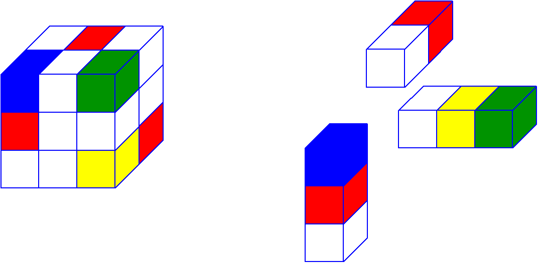
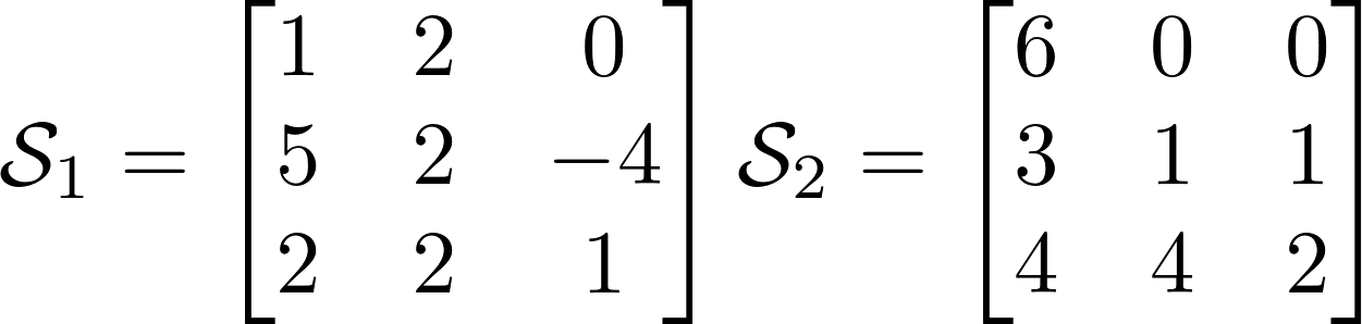
Let's immediately give an example of a third order tensor. Meet with this tensor today you will work and you will see a bit of tensor magic on it. I wrote his frontal sections below.
')
Linear algebra defines to us the product between two matrices as follows:

In this work, two dimensions are specified and the operation between objects with dimensions greater than two is not defined. Tensor algebra gives tools how to get around this restriction, using the features of more spaces in linear algebra. To begin, I will introduce three matrix operations, without which you cannot step in tensor algebra and step:
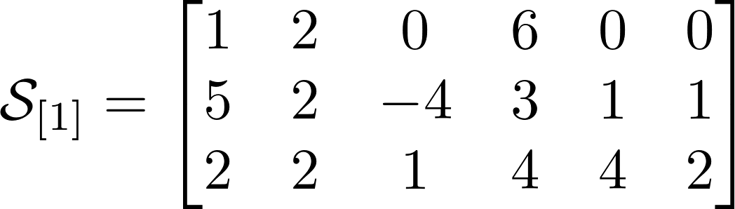
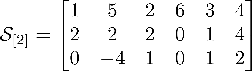
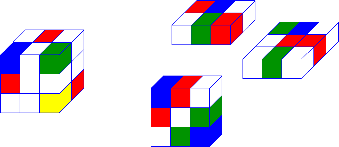
In tensor algebra, one of the key concepts is “unfolding” (I will call it a sweep to reduce anglicisms) or the representation of a tensor through a matrix. A sweep is a mapping of a tensor to one of its spaces. The tensor in this operation is recorded as a matrix, the number of rows of which is equal to the number of elements of the developed space. Elements in the row have the same sequence number for the specified space.
The number of possible sweeps is equal to the order of the tensor or its dimension. The tensor from our example has 3 sweeps. Above are the sweeps for our tensor, and I hope it will be much easier for you to understand them than for explanations. Tensors seemed to me much clearer in an intuitive sense, rather than by definition.
The next operation I want to describe is the product of a tensor with a matrix in a given space. It is written in the following way and in essence it is the product of two matrices, where the right-hand matrix is the development of the tensor in the multiplied space, and on the left the matrix with which is actually multiplied.
The important point is that the multiplication is written to the right, and happens to the left of the tensor. The result is a matrix which is a scan of the new tensor, which can be assembled back into the usual tensor. It is important to note that as a result of this operation, the dimension of the space with which the multiplication occurs can change , the others cannot . Example below

The unit rank tensor is such a tensor of dimension N , which can be obtained by multiplying one by N vectors, one for each space. How it looks visually for the third-order tensor I showed below. A unit rank tensor is analogous to a single component for an SVD matrix, where a complex matrix is decomposed into unit rank matrices. A unit rank tensor can be both complex and real, depending on the requirements we make to it.

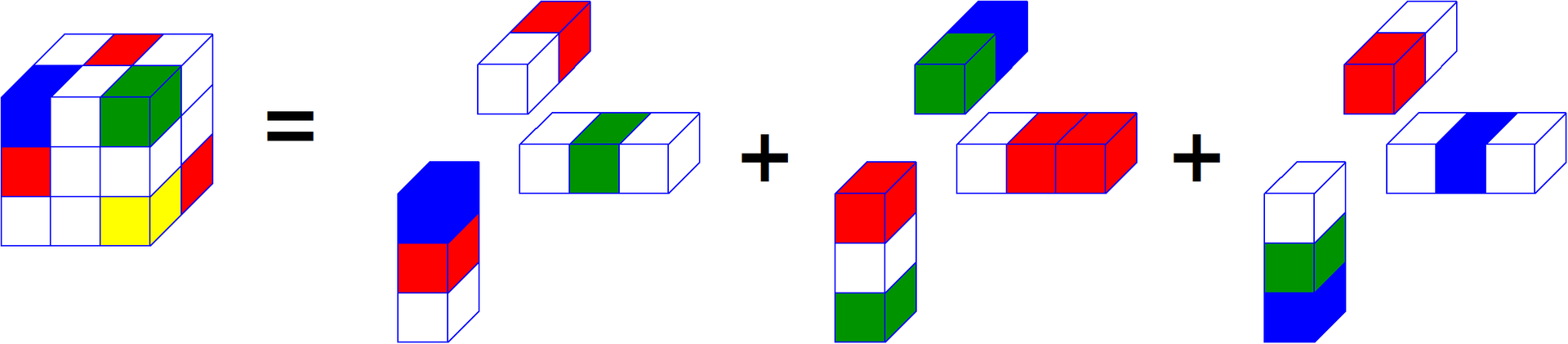
The most important and interesting in tensors is their decomposition. I hope many of you know or have heard about decomposition of a matrix into singular values. With it, we can present the matrix as the sum of matrices of unit rank, and evaluate their contribution to the common matrix. Below is an example of such a decomposition.
There is a very similar analogue in tensor algebra and it is called “CP”, it is also called “CANDECOMP” or “PARAFAC”. “CP” decomposes any tensor for the sum of unit rank tensors. This formulation has two forms of notation, the simplest of which actually records the tensor as the sum of the set of tensors of unit rank, while the other writes the decomposition through matrices in each of the spaces. In addition to the decomposition of "CP" in tensor algebra there are a large number of its analogues, depending on the valuation of the components and other features.
Look, if you write the vectors of each of the spaces one by one, you will get N matrices. Each of the matrices represents a certain “basis” in its space. This form of recording resembles the SVD matrix. From these matrices one can get back the tensor, if we take the unit tensor and alternately multiply it by all matrix bases in the spaces.

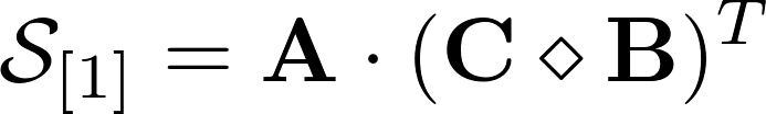
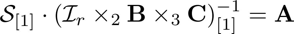
From the decomposition of the third-order tensor, it is easy to derive a sweep expression; it will allow one of the matrices to be separated by the usual matrix product. Look below, see, the matrix A is recorded through a work with a different matrix, which in turn is a product of the work of Khatri-Rao. Knowing the product of the product and the initial scan, we can calculate the matrix A using linear algebra. This greatly simplifies the work of the decomposition calculation algorithms for third order tensors and gives convenient formulas for iterations.
Why do we need this nonsense, we could do the SVD sweep? Of course they could, but in the general case the decomposition of the tensor makes it much easier to describe the data, it becomes easier to compress or find patterns. This is especially important for large amounts of data, since with increasing dimensions, the rank changes much less.
This expansion, for all its charms, has two problems. First: the rank of this expansion you need to know for yourself. This is often a non-trivial task, especially if the data has noise.
The second problem is the calculation of the decomposition itself. The most common algorithm at the moment is ALS or PMNK . There is also an algorithm with the romantic name SECSI , but I will probably tell about it in the future. PMNK or interleaved least squares method is simple to disgrace, it has the following algorithm:

The drawbacks of this method are a great many, these are local minima, and computational complexity, but it still remains one of the most used algorithms at the present time.
And now let's move closer to GFDM technology. There is another decomposition called PARATUCK2, and this is an abbreviation for the other two abbreviations "PARAFAC" and "TUCKER2". Yes, an abbreviation consisting of two other abbreviations, how wonderful it is.
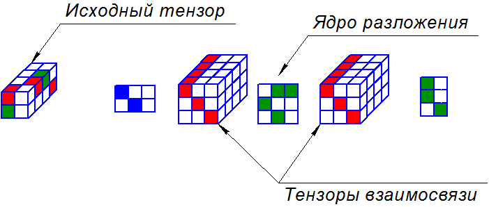
This decomposition writes the tensor through three matrices and two tensors. The matrix in the middle is called the decomposition kernel, the tensors are called unifying. Extreme two matrices have no special name. How to calculate the tensor from this expansion is a separate story.
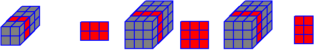
The tensor from the decomposition is considered in layers, in each layer only the corresponding layer of interrelation tensors is selected. As a result, 5 matrices are obtained, multiplying which we obtain the values of the tensor. This operation is repeated for each of the layers, and the results are collected one by one. The number of rows of the first matrix is equal to the number of rows of the tensor, similarly with the columns of the third matrix and tensor, as well as with the depth of interrelation tensors. It was very difficult for me to understand at the first moment. And what is most interesting, this model can really help you with data analysis.
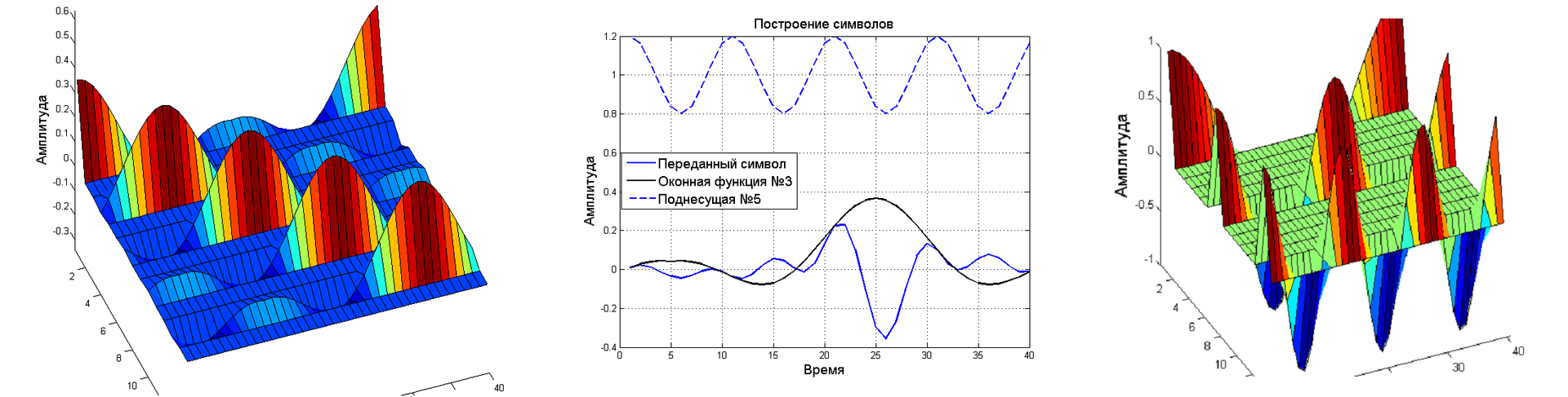
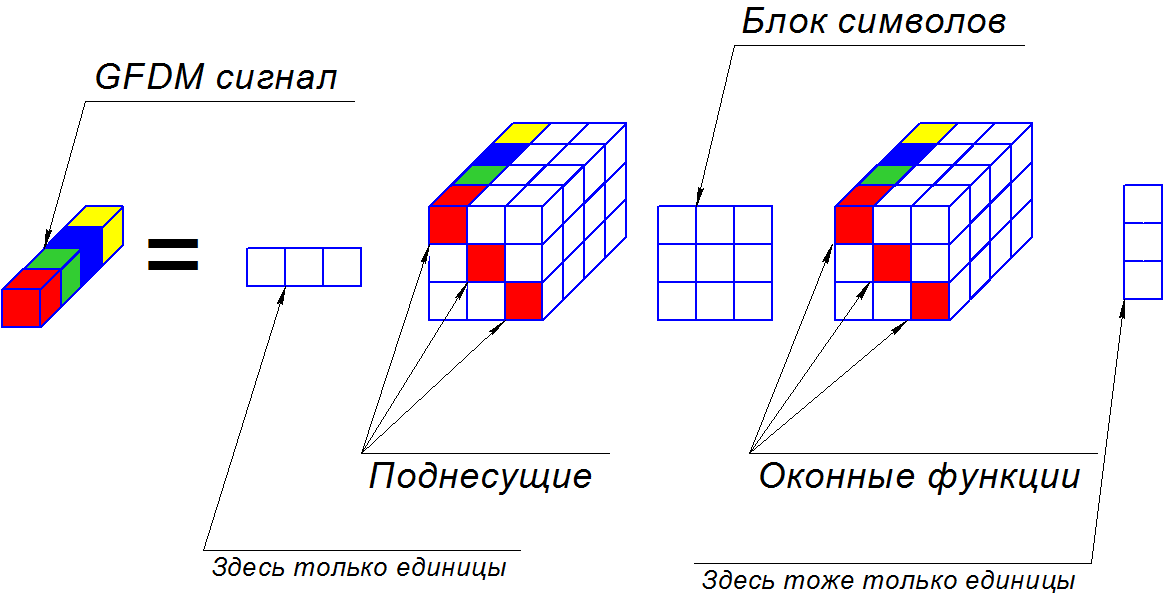
So why do we need this decomposition? It is quite complex and consists of five elements, how can it even help with GFDM? Let's first recall and fix a bit about GFDM. Below is the symbol generation method that the transmitter sends. A data block can be formed as a matrix, where the rows are subcarriers, and the columns are temporary positions in the block. The total data block is obtained by summing all the elements, in other words, it is necessary to multiply the element-wise vector of the subcarrier with the vector of the window function, and all this by the symbol that we transmit. Thus, each symbol is located at the intersection of two vectors with which it is multiplied. The operation is quite simple, but it is difficult to describe it through the product of the modulation matrix and the vector of symbols. The form of the record through the modulation matrix is the main building block for building receivers.
If you take a closer look, PARATUCK2 can really describe GFDM. To do this, we need to take the vector row and column vector as the extreme matrices, and add window functions and subcarriers to the relationship tensors along the main diagonals. If symbols appear in the core matrix, the result will be a vector in the third dimension and correspond to the transmitted data.
Famously wrapped, is not it? When I was writing a diploma, it was difficult to understand how this can be simplified and brought to an acceptable form, but it is possible! Through this decomposition, one can simplify the expression of the modulation matrix into the product of two matrices. However, I think to tell the next time, along with the theory of Zero-forcing, Matched filter and Minimal Mean squared error receivers.
Have a nice week.
Part 1 here
Abbreviations
CP - CANDECOMP / PARAFAC
CANDECOMP - Canonical decomposition
PARAFAC - parallel Factors
PARATCUK2 - PARAFAC / Tucker2
ALS - Alternating least squares
PMNK - interleaved least squares method
SVD - Singular value decomposition
SLAU - System of linear algebraic equations
GFDM - generalized frequency division multiplexing
SECSI - SEmi-algebraic framework for approximat eCP decompositions via SImultaneous Matrix Diagonalizations
Used notation
As lowercase letters without bold type, scalar values are indicated. Like this:

As lowercase letters in bold type, vectors are indicated. Like this:

Matrices are indicated as uppercase letters in bold. Like this:

As uppercase calligraphic letters denoted by tensors. Like this:

Subscripts indicate the position in the matrix in rows and columns.
In scans, subscript characters inform about the space being deployed.
Subscript characters in tensors inform about the frontal section of the tensor, unless otherwise specified.

As lowercase letters in bold type, vectors are indicated. Like this:
Matrices are indicated as uppercase letters in bold. Like this:
As uppercase calligraphic letters denoted by tensors. Like this:
Subscripts indicate the position in the matrix in rows and columns.
In scans, subscript characters inform about the space being deployed.
Subscript characters in tensors inform about the frontal section of the tensor, unless otherwise specified.
Tensors
Perhaps the best definition of a tensor would be the quote of Tamara G. Kolda:
A tensor is a multidimensional arrayThere is simply no place. Ideas with tensors arose initially in linear algebra. Therefore, the best way is to describe everything using linear algebra. In linear algebra, we use scalars, vectors, matrices, and we can perform addition, subtraction, and multiplication operations. The scalar consists of 1 element, the vector consists of N elements and the matrix consists of MN elements. Tensors include everything that linear algebra can and even a bit more. Giving examples from linear algebra: a vector is a first-order tensor, and a matrix is a second-order tensor. Consequently, the order of the tensor is determined by the number of spaces in which the tensor has more than one element. The more spaces you have, the higher the order of the tensor is. Simple enough, right?
Let's immediately give an example of a third order tensor. Meet with this tensor today you will work and you will see a bit of tensor magic on it. I wrote his frontal sections below.
')
Linear algebra defines to us the product between two matrices as follows:
In this work, two dimensions are specified and the operation between objects with dimensions greater than two is not defined. Tensor algebra gives tools how to get around this restriction, using the features of more spaces in linear algebra. To begin, I will introduce three matrix operations, without which you cannot step in tensor algebra and step:
Kronecker's work
So, in the Kronecker product (or as it is also called the tensor product) two matrices are involved, the result of their work will be a block matrix, each block of which is the second matrix multiplied by a certain element of the first matrix.

This operation is used to form a simplified channel model in MIMO.
This operation is used to form a simplified channel model in MIMO.
artwork Khatri-Rao
The Khatri-Rao product is denoted by the following symbol and is a Kronecker product for all the corresponding columns. In other words, each i- th column from matrix A is multiplied by the i- th column of matrix B and the result is the i-th column of the resulting matrix.

This operation is most often used in third order tensors, for example through it I described the modulation matrix of the GFDM system.
This operation is most often used in third order tensors, for example through it I described the modulation matrix of the GFDM system.
Hadamard's Work
The Hadamard product is the simplest of all, it is an elementwise product of all positions in the matrices A and B.

Basic operations in tensor algebra
Scan
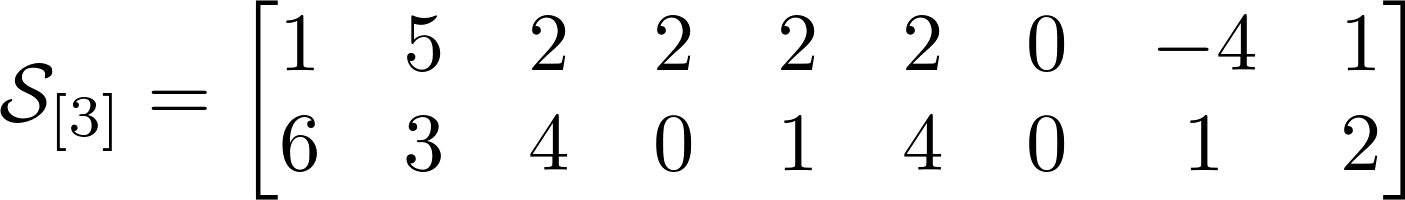
In tensor algebra, one of the key concepts is “unfolding” (I will call it a sweep to reduce anglicisms) or the representation of a tensor through a matrix. A sweep is a mapping of a tensor to one of its spaces. The tensor in this operation is recorded as a matrix, the number of rows of which is equal to the number of elements of the developed space. Elements in the row have the same sequence number for the specified space.
Feature
There are two types of recording elements in a line: according to the Lauer notation and according to the Matlab notation. The most commonly used notation is Matlab, so I will use it. According to the Matlab notation, elements go in ascending order in dimension, i.e. first comes the element in the first dimension, then in the second, and so on, excluding the unfolding dimension.
The number of possible sweeps is equal to the order of the tensor or its dimension. The tensor from our example has 3 sweeps. Above are the sweeps for our tensor, and I hope it will be much easier for you to understand them than for explanations. Tensors seemed to me much clearer in an intuitive sense, rather than by definition.
The product of a given space
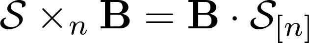
The next operation I want to describe is the product of a tensor with a matrix in a given space. It is written in the following way and in essence it is the product of two matrices, where the right-hand matrix is the development of the tensor in the multiplied space, and on the left the matrix with which is actually multiplied.
The important point is that the multiplication is written to the right, and happens to the left of the tensor. The result is a matrix which is a scan of the new tensor, which can be assembled back into the usual tensor. It is important to note that as a result of this operation, the dimension of the space with which the multiplication occurs can change , the others cannot . Example below
Unit Rank Tensor
The unit rank tensor is such a tensor of dimension N , which can be obtained by multiplying one by N vectors, one for each space. How it looks visually for the third-order tensor I showed below. A unit rank tensor is analogous to a single component for an SVD matrix, where a complex matrix is decomposed into unit rank matrices. A unit rank tensor can be both complex and real, depending on the requirements we make to it.
Decomposition of tensors
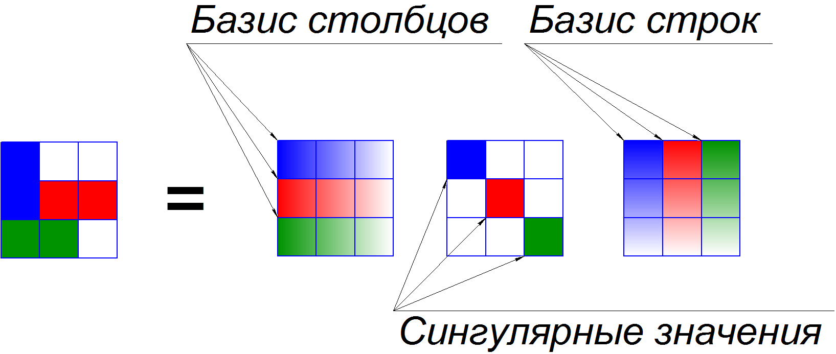
The most important and interesting in tensors is their decomposition. I hope many of you know or have heard about decomposition of a matrix into singular values. With it, we can present the matrix as the sum of matrices of unit rank, and evaluate their contribution to the common matrix. Below is an example of such a decomposition.
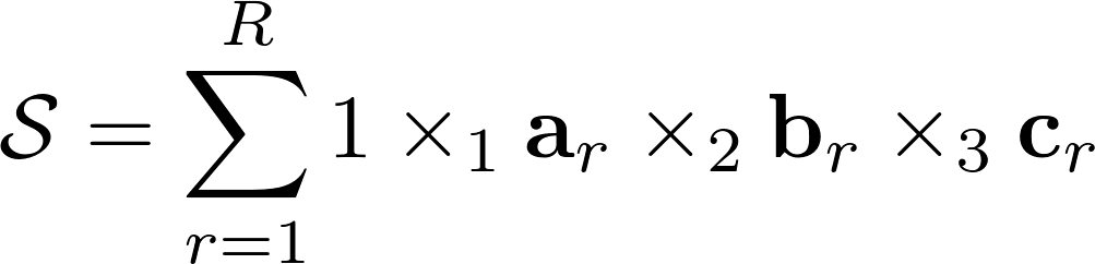
There is a very similar analogue in tensor algebra and it is called “CP”, it is also called “CANDECOMP” or “PARAFAC”. “CP” decomposes any tensor for the sum of unit rank tensors. This formulation has two forms of notation, the simplest of which actually records the tensor as the sum of the set of tensors of unit rank, while the other writes the decomposition through matrices in each of the spaces. In addition to the decomposition of "CP" in tensor algebra there are a large number of its analogues, depending on the valuation of the components and other features.
Look, if you write the vectors of each of the spaces one by one, you will get N matrices. Each of the matrices represents a certain “basis” in its space. This form of recording resembles the SVD matrix. From these matrices one can get back the tensor, if we take the unit tensor and alternately multiply it by all matrix bases in the spaces.
From the decomposition of the third-order tensor, it is easy to derive a sweep expression; it will allow one of the matrices to be separated by the usual matrix product. Look below, see, the matrix A is recorded through a work with a different matrix, which in turn is a product of the work of Khatri-Rao. Knowing the product of the product and the initial scan, we can calculate the matrix A using linear algebra. This greatly simplifies the work of the decomposition calculation algorithms for third order tensors and gives convenient formulas for iterations.
Why do we need this nonsense, we could do the SVD sweep? Of course they could, but in the general case the decomposition of the tensor makes it much easier to describe the data, it becomes easier to compress or find patterns. This is especially important for large amounts of data, since with increasing dimensions, the rank changes much less.
Decomposition problems
This expansion, for all its charms, has two problems. First: the rank of this expansion you need to know for yourself. This is often a non-trivial task, especially if the data has noise.
An example from my experience
The ordinate represents the normalized recovery error and the abscissa used is the rank of the decomposition. I only decomposed the tensor with the sum of the signal and noise and only noise. The assumption of rank had to be made only by the unusual behavior of the error of expansion. Attention, the legend is confused.
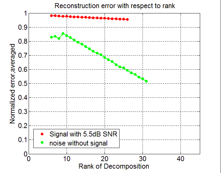
The algorithm was to search for a GPS signal when calculating the correlation by the polyphase Fourier transform. In this case, the dimension of the output data on the correlator was equal to four (time, frequency, code, shift of the polyphase transformation).
The algorithm was to search for a GPS signal when calculating the correlation by the polyphase Fourier transform. In this case, the dimension of the output data on the correlator was equal to four (time, frequency, code, shift of the polyphase transformation).
The second problem is the calculation of the decomposition itself. The most common algorithm at the moment is ALS or PMNK . There is also an algorithm with the romantic name SECSI , but I will probably tell about it in the future. PMNK or interleaved least squares method is simple to disgrace, it has the following algorithm:
- Set the rank of the expansion
- We generate random decomposition matrices of spaces.
- We fix all matrices except one and calculate the remaining matrix with the help of SLAE
- Repeat the previous paragraph for all matrices in turn, until the discrepancy becomes acceptable
The drawbacks of this method are a great many, these are local minima, and computational complexity, but it still remains one of the most used algorithms at the present time.
GFDM communication
And now let's move closer to GFDM technology. There is another decomposition called PARATUCK2, and this is an abbreviation for the other two abbreviations "PARAFAC" and "TUCKER2". Yes, an abbreviation consisting of two other abbreviations, how wonderful it is.
This decomposition writes the tensor through three matrices and two tensors. The matrix in the middle is called the decomposition kernel, the tensors are called unifying. Extreme two matrices have no special name. How to calculate the tensor from this expansion is a separate story.
The tensor from the decomposition is considered in layers, in each layer only the corresponding layer of interrelation tensors is selected. As a result, 5 matrices are obtained, multiplying which we obtain the values of the tensor. This operation is repeated for each of the layers, and the results are collected one by one. The number of rows of the first matrix is equal to the number of rows of the tensor, similarly with the columns of the third matrix and tensor, as well as with the depth of interrelation tensors. It was very difficult for me to understand at the first moment. And what is most interesting, this model can really help you with data analysis.
So why do we need this decomposition? It is quite complex and consists of five elements, how can it even help with GFDM? Let's first recall and fix a bit about GFDM. Below is the symbol generation method that the transmitter sends. A data block can be formed as a matrix, where the rows are subcarriers, and the columns are temporary positions in the block. The total data block is obtained by summing all the elements, in other words, it is necessary to multiply the element-wise vector of the subcarrier with the vector of the window function, and all this by the symbol that we transmit. Thus, each symbol is located at the intersection of two vectors with which it is multiplied. The operation is quite simple, but it is difficult to describe it through the product of the modulation matrix and the vector of symbols. The form of the record through the modulation matrix is the main building block for building receivers.
If you take a closer look, PARATUCK2 can really describe GFDM. To do this, we need to take the vector row and column vector as the extreme matrices, and add window functions and subcarriers to the relationship tensors along the main diagonals. If symbols appear in the core matrix, the result will be a vector in the third dimension and correspond to the transmitted data.
Example from experience
Initially, I additionally intended to describe the frequency-dependent channel through the values in the vector next to the subcarrier tensor. This was an erroneous assumption.
Famously wrapped, is not it? When I was writing a diploma, it was difficult to understand how this can be simplified and brought to an acceptable form, but it is possible! Through this decomposition, one can simplify the expression of the modulation matrix into the product of two matrices. However, I think to tell the next time, along with the theory of Zero-forcing, Matched filter and Minimal Mean squared error receivers.
References
TG Kolda and BW Bader, \ Tensor decompositions and applications, "SIAM Review,
vol. 51, no. 3, pp. 455 {500, 2009.
R. Bro, N. Sidiropoulos, and G. Giannakis, \ Parafac: Tutorial and applications, "
Chemometrics Group, Food Technology, Royal Veterinary Agricultural University, 1997.
L. de Lathauwer, B. de Moor, and J. Vanderwalle, \ A multilinear singular value decom-
position, "SIAM J. MATRIX ANAL. APPL. Vol. 21, No. 4, pp. 1253 1278, 2000.
KB Petersen and MS Pedersen, The Matrix Cookbook. Petersen & Pedersen ,, 2012.
S. LIU and G. TRENKLER, \ Hadamard, khatri-rao, kronecker and other matrix
products, "INTERNATIONAL JOURNAL OF INFORMATION AND SYSTEMS SCI-
ENCES, 2006.
ALF de Almeida, G. Favier, and LR Ximenes, \ Space-time-frequency (stf) mimo
paratuck2 model, "
IEEE Transaction in signal processing, vol. 61, no. 8 ,, APR, 2013.
Have a nice week.
Source: https://habr.com/ru/post/369925/
All Articles