Self-test MEMS accelerometer, gyro and compass (self test)
Studying the specification (datasheet) for the MEMS sensor (accelerometer, gyroscope, etc.) we are faced with a procedure such as self-test (self-test) or self-diagnosis. Usually in the specifications there is a description of how to do it. Who cares: what is it and how to do it right? - welcome under cat.

The self-test allows you to determine that the data from the sensor shows what should be shown. Sensors do not always have a self-test mode. To determine the conformity of the measured data to what is stated in the specification, the developer had to check this with special experiments. In the case of an accelerometer, tilt at certain angles and take a change in readings. Analyzing the results, it was possible to estimate the error produced by the sensor. If the indicators did not meet the specifications, the sensor was recognized as defective.
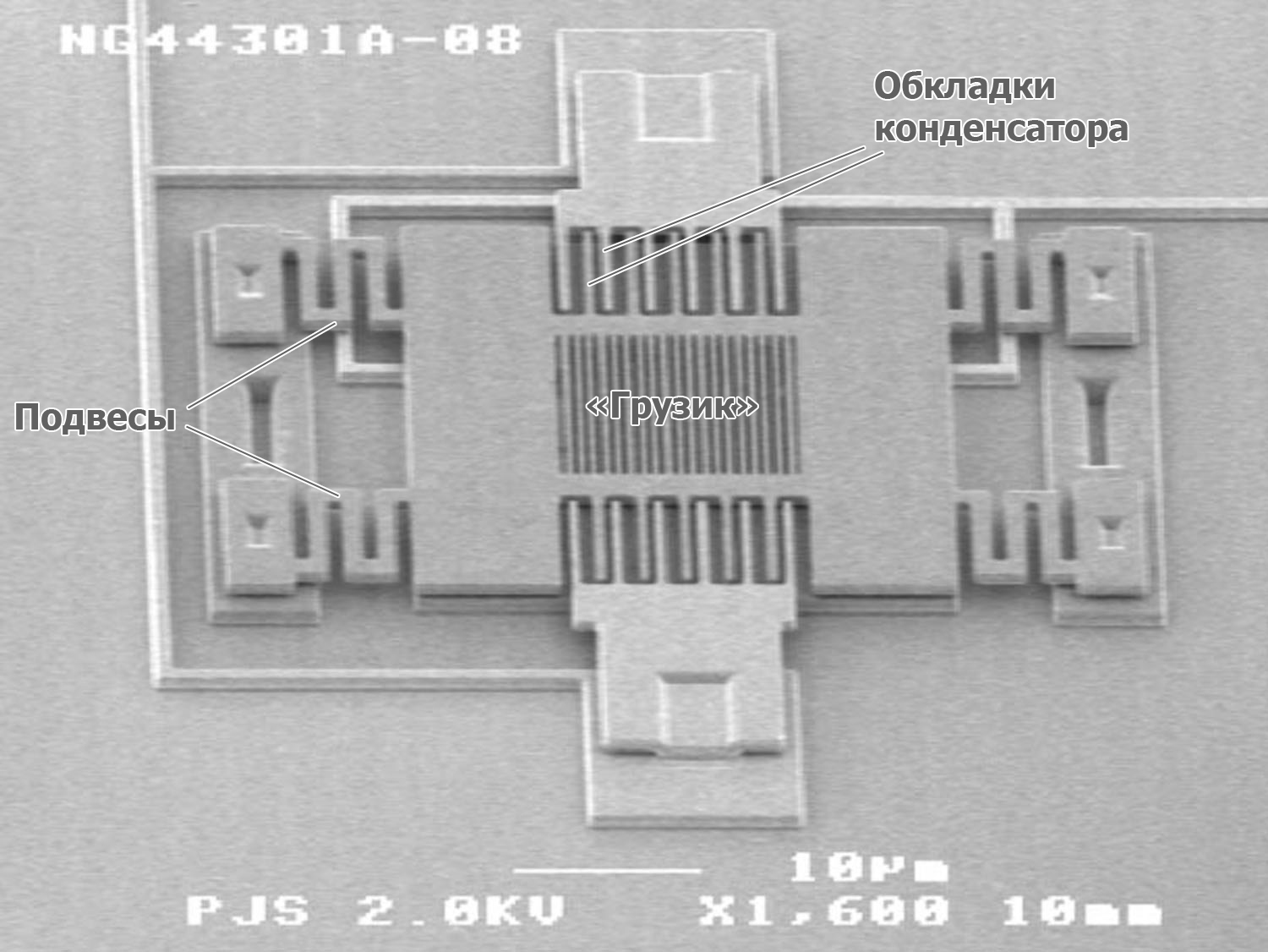
This complicated the mass production and began to include a self-diagnostic procedure in all sensors. The plan of the procedure is quite simple - to create conditions under which we will know what the sensor should show, and compare it with what it shows. Deviations higher than specified reject the sensor. For compasses, they make an element that creates a magnetic field (right in the sensor case). The inclusion of self-diagnosis mode includes this element - the reference source. For an accelerometer and a gyroscope, the element generates an electrostatic field that deflects the weight (see photo below) and simulates physical movement or rotation. The amount of displacement is known, respectively, the value that the sensor should show is known. If the error of the readings is within the stated limits, then the sensor is OK and it works in accordance with the specification.
')
(an article from an online magazine from which I borrowed a picture contains many more beautiful enlarged photos, see links below)
Consider the accelerometer. As mentioned earlier, in the self-test mode, the electromechanical weight is affected by an electrostatic force, which deflects it at a certain distance, and thus simulates acceleration. However, the expected value at the output of the sensor, we will not see. The fact is that in a calm state other forces act on a small weight (for example, gravity). They additionally reject the weight.
In order to take into account external forces, in the self-test procedure, the sensor readings are taken in the normal mode. Then the deviation source is switched on (switching to the “self-test” mode) and the sensor readings are again taken.
a norm = a external
a ST = a external + a int. ist
The difference in the readings of these two modes should show the value from the reference source. If the value is within the specification range, this means that the sensor is working properly.
a ext. ist = a ST - a norm
MIN <a int. ist <Max
From here an important conclusion - external forces in both modes should be equal. That is, the sensor must be fixed. When the device is in the hands - it is movable. When you press something (or finish pressing) on the device, it is also mobile. If the device is vibrated, it is mobile. And so on.
When conducting a self-test sensor also need to consider:
The deviation of the weight of the reference source for the axes:
The magnitude of the deviation is usually indicated in arbitrary units of the sensor - LSB. This is what lies in the output register. Consider the values given by the internal source of the LIS302DL sensor (8-bit sensor):
It is interesting because it contains two modes of operation of the internal source. Looking at the table one might think that the values are given for both directions of the internal source. However, in reality this is an extended range for one direction - “Self test P”. Usually the direction is one and the values are indicated as follows:
Or you can specify in measured units:
To get the measured value from the sensor values, you need to use the formula:
Value_in_units_measurement = Value_in_LSB * Sensitivity.
To convert the measured value back to the sensor unit, you need to use the formula:
Value_in_LSB = Value_in_units_measures / Sensitivity.
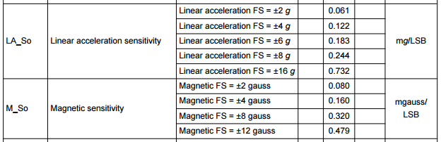
The sensitivity in the specifications is as follows:

or so
You can calculate the sensitivity yourself:
Sensitivity = Measured_band / Resolution
Example: Value_LSB = Size_measurable * Resolution / Measurement_band = 8 * 0.001 * g * 65536/4 * g = 131.072, i.e. ± 131.
The valid range can be specified in several ways:
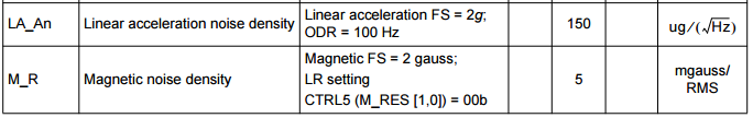
The noise level is usually indicated by the standard deviation (RMS). The range of error will then be equal to twice the standard deviation (±). Examples:

In the first example, the root of the spectral power density of the noise is indicated. To get the MSE of the noise, the value should be multiplied by the root of the filter band, which you will have on the sensor output. For example, if the band is 25 Hz, get 750 ug as the standard deviation (thanks to Korogodin for the hint). If we want to get the value without filtering, we take the frequency of measurements. In this case, at 100 Hz, 1.5mg is obtained. In the second and third example, the maximum noise level is indicated. For example, 8 * 0.001 * g = 0.0784 m / s 2 . This means a possible run-up of self-test = ± 0.0784 m / s 2 . Here you also need to be careful, because sometimes the noise level is indicated with the filter turned on. This means that measurements need to be done with the same filter settings.
Examples of self-diagnosis:
Introduction
The self-test allows you to determine that the data from the sensor shows what should be shown. Sensors do not always have a self-test mode. To determine the conformity of the measured data to what is stated in the specification, the developer had to check this with special experiments. In the case of an accelerometer, tilt at certain angles and take a change in readings. Analyzing the results, it was possible to estimate the error produced by the sensor. If the indicators did not meet the specifications, the sensor was recognized as defective.
This complicated the mass production and began to include a self-diagnostic procedure in all sensors. The plan of the procedure is quite simple - to create conditions under which we will know what the sensor should show, and compare it with what it shows. Deviations higher than specified reject the sensor. For compasses, they make an element that creates a magnetic field (right in the sensor case). The inclusion of self-diagnosis mode includes this element - the reference source. For an accelerometer and a gyroscope, the element generates an electrostatic field that deflects the weight (see photo below) and simulates physical movement or rotation. The amount of displacement is known, respectively, the value that the sensor should show is known. If the error of the readings is within the stated limits, then the sensor is OK and it works in accordance with the specification.
')
(an article from an online magazine from which I borrowed a picture contains many more beautiful enlarged photos, see links below)
1. Influence of external forces on self-testing
Consider the accelerometer. As mentioned earlier, in the self-test mode, the electromechanical weight is affected by an electrostatic force, which deflects it at a certain distance, and thus simulates acceleration. However, the expected value at the output of the sensor, we will not see. The fact is that in a calm state other forces act on a small weight (for example, gravity). They additionally reject the weight.
In order to take into account external forces, in the self-test procedure, the sensor readings are taken in the normal mode. Then the deviation source is switched on (switching to the “self-test” mode) and the sensor readings are again taken.
a norm = a external
a ST = a external + a int. ist
The difference in the readings of these two modes should show the value from the reference source. If the value is within the specification range, this means that the sensor is working properly.
a ext. ist = a ST - a norm
MIN <a int. ist <Max
From here an important conclusion - external forces in both modes should be equal. That is, the sensor must be fixed. When the device is in the hands - it is movable. When you press something (or finish pressing) on the device, it is also mobile. If the device is vibrated, it is mobile. And so on.
2. What else needs to be considered when conducting a self-test?
When conducting a self-test sensor also need to consider:
- When switching the sensor to the measurement mode, it may take a certain amount of time for the accelerometer to become ready for data collection. Time to specify in the specification.
- Carrying out self-diagnostics is preferably carried out in different measured ranges of the sensor (2G, 4G, etc.).
- Sometimes it is possible the inversion of the reference source (can pull in one direction or the other). The specification will then indicate two self-test modes (for example, “Self-test P (ositive)” and “Self-test N (egative)”).
3. How to find the deviation of the weight of the reference source?
The deviation of the weight of the reference source for the axes:
- May be specified explicitly in the specification.
- A wide range of possible values can be specified. The principle is the same - if the difference obtained is a int. ist falls into this range, then the sensor is OK. It is only necessary to understand that this approach is not practiced for the most accurate sensors.
- Values can be stored in special registers (something like "SELF_TEST_X_ACCEL"). This means the manufacturer specified the deviation values for each specific sensor and put in its memory. The manufacturer can save memory and write not the value, but the coefficient of the formula with which the value can be calculated. The calculation method itself will then be in the specification or in one of its applications.
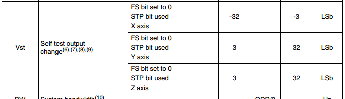
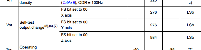
The magnitude of the deviation is usually indicated in arbitrary units of the sensor - LSB. This is what lies in the output register. Consider the values given by the internal source of the LIS302DL sensor (8-bit sensor):
It is interesting because it contains two modes of operation of the internal source. Looking at the table one might think that the values are given for both directions of the internal source. However, in reality this is an extended range for one direction - “Self test P”. Usually the direction is one and the values are indicated as follows:
Or you can specify in measured units:
To get the measured value from the sensor values, you need to use the formula:
Value_in_units_measurement = Value_in_LSB * Sensitivity.
To convert the measured value back to the sensor unit, you need to use the formula:
Value_in_LSB = Value_in_units_measures / Sensitivity.
The sensitivity in the specifications is as follows:
or so
You can calculate the sensitivity yourself:
Sensitivity = Measured_band / Resolution
Example: Value_LSB = Size_measurable * Resolution / Measurement_band = 8 * 0.001 * g * 65536/4 * g = 131.072, i.e. ± 131.
4. How to understand that the value is in the acceptable range?
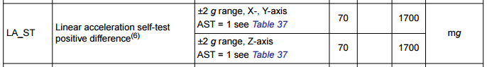
The valid range can be specified in several ways:
- Can be explicitly specified minimum and maximum.
- It can be specified as a percentage tolerance (for example, somewhere in the footnote).
- The idea should be no more than the noise level.
The noise level is usually indicated by the standard deviation (RMS). The range of error will then be equal to twice the standard deviation (±). Examples:
In the first example, the root of the spectral power density of the noise is indicated. To get the MSE of the noise, the value should be multiplied by the root of the filter band, which you will have on the sensor output. For example, if the band is 25 Hz, get 750 ug as the standard deviation (thanks to Korogodin for the hint). If we want to get the value without filtering, we take the frequency of measurements. In this case, at 100 Hz, 1.5mg is obtained. In the second and third example, the maximum noise level is indicated. For example, 8 * 0.001 * g = 0.0784 m / s 2 . This means a possible run-up of self-test = ± 0.0784 m / s 2 . Here you also need to be careful, because sometimes the noise level is indicated with the filter turned on. This means that measurements need to be done with the same filter settings.
Examples of self-diagnosis:
LSM303D self-test code example
In one position, the following results were obtained:
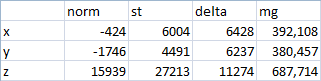
Then I put the board with the sensor on its side and got the following results:
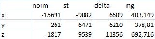
The run-up of values turned out to be 11, 2 and 5 g * 10 -3 . If you conduct a few more tests, you can specify the range for this particular sensor:
380 <X <410
370 <Y <390
680 <Z <700
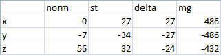
uint8_t sign = lsm303d_read(LSM303D_ADDR_WHO_AM_I); if (sign != LSM303D_WHO_I_AM) { //on_fatal_error(" LSM303D"); } lsm303d_write(LSM303D_ADDR_CTRL_REG1, LSM303D_REG1_RATE_100HZ_A | LSM303D_REG1_X_ENABLE_A | LSM303D_REG1_Y_ENABLE_A | LSM303D_REG1_Z_ENABLE_A ); delay_ms(100); uint8_t i; int32_t avg_x__norm = 0, avg_y__norm = 0, avg_z__norm = 0; vector v; // 100 for (i = 0; i < 100; i++) { lsm303d_get_acc(&v); avg_x__norm += vx; avg_y__norm += vy; avg_z__norm += vz; } avg_x__norm /= 100; avg_y__norm /= 100; avg_z__norm /= 100; // ( "self-test") lsm303d_write(LSM303D_ADDR_CTRL_REG2, LSM303D_REG2_FULL_SCALE_2G_A | 2 ); delay_ms(100); int32_t avg_x__st = 0, avg_y__st = 0, avg_z__st = 0; // 100 for (i = 0; i < 100; i++) { lsm303d_get_acc(&v); avg_x__st += vx; avg_y__st += vy; avg_z__st += vz; } avg_x__st /= 100; avg_y__st /= 100; avg_z__st /= 100; // lsm303d_write(LSM303D_ADDR_CTRL_REG2, 0); delay_ms(100); float internal_source_x, internal_source_y, internal_source_z; // mg internal_source_x = (avg_x__st - avg_x__norm)*0.061; internal_source_y = (avg_y__st - avg_y__norm)*0.061; internal_source_z = (avg_z__st - avg_z__norm)*0.061; if ((internal_source_x < 70.0) || (internal_source_x >1700.0) || (internal_source_y < 70.0) || (internal_source_y >1700.0) || (internal_source_z < 70.0) || (internal_source_z >1700.0)) { // detect problem draw_EraseScreen(); draw_TextOut(0,0,"problem.."); draw_Show(); } else { draw_EraseScreen(); draw_TextOut(0,0,"ok"); draw_Show(); } while(1); In one position, the following results were obtained:
Then I put the board with the sensor on its side and got the following results:
The run-up of values turned out to be 11, 2 and 5 g * 10 -3 . If you conduct a few more tests, you can specify the range for this particular sensor:
380 <X <410
370 <Y <390
680 <Z <700
LIS302DL Self Test Code Example
In one position, the following results were obtained:

In another position, these results:

The run-up of values turned out to be around 1 unit And this is the second mode of operation of the internal source, when it pulls in the other direction (Self-test M):
Here we see the readings of another sensor (“Self-test P”):
And the second mode with the rotation of the board ("Self-test M"):
According to the specification, it does not pass a self-test - the values along the Z axis stand for the stated limit: a maximum of 32, and we have 35.
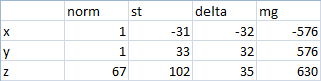
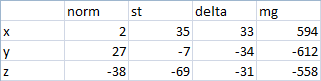
uint8_t dev_id = lis302dl_read(0x0F); if (dev_id != 0x3b) { while(1); // } lis302dl_write(0x20, 7 | // // 100 2G (1 << 6) // ); delay_ms(100); uint8_t i; int32_t avg_x__norm = 0, avg_y__norm = 0, avg_z__norm = 0; // 100 for (i = 0; i < 100; i++) { lis302dl_get_acc(&v); avg_x__norm += vx; avg_y__norm += vy; avg_z__norm += vz; } avg_x__norm /= 100; avg_y__norm /= 100; avg_z__norm /= 100; // ( "self-test P") lis302dl_write(0x20, 7 | // (1 << 4) | // self-test P // 100 2G (1 << 6) // ); delay_ms(100); int32_t avg_x__st = 0, avg_y__st = 0, avg_z__st = 0; // 100 for (i = 0; i < 100; i++) { lis302dl_get_acc(&v); avg_x__st += vx; avg_y__st += vy; avg_z__st += vz; } avg_x__st /= 100; avg_y__st /= 100; avg_z__st /= 100; // lis302dl_write(0x20, 7 | // // 100 2G (1 << 6) // ); delay_ms(100); int32_t internal_source_x, internal_source_y, internal_source_z; // LSB internal_source_x = avg_x__st - avg_x__norm; internal_source_y = avg_y__st - avg_y__norm; internal_source_z = avg_z__st - avg_z__norm; if ((internal_source_x < -32) || (internal_source_x > -3) || (internal_source_y < 3) || (internal_source_y > 32) || (internal_source_z < 3) || (internal_source_z > 32)) { // detect problem draw_EraseScreen(); draw_TextOut(0,0,"problem.."); draw_Show(); } else { draw_EraseScreen(); draw_TextOut(0,0,"ok"); draw_Show(); } while(1); In one position, the following results were obtained:
In another position, these results:
The run-up of values turned out to be around 1 unit And this is the second mode of operation of the internal source, when it pulls in the other direction (Self-test M):
Here we see the readings of another sensor (“Self-test P”):
And the second mode with the rotation of the board ("Self-test M"):
According to the specification, it does not pass a self-test - the values along the Z axis stand for the stated limit: a maximum of 32, and we have 35.
MPU9250 self-test code example
In one position, the following results were obtained:
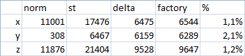
In another position:
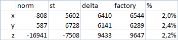
In this sensor, the success of the self-test is determined by the permissible deviation from the reference value. The tolerance of the deviation is ± 3% (p. 9 of the first part of the specification). That is, this sensor is fine.
delay_ms(100); uint8_t i; int32_t avg_x__norm = 0, avg_y__norm = 0, avg_z__norm = 0; // 100 for (i = 0; i < 100; i++) { mpu9250_get_acc(&v); avg_x__norm += vx; avg_y__norm += vy; avg_z__norm += vz; } avg_x__norm /= 100; avg_y__norm /= 100; avg_z__norm /= 100; // ( "self-test") mpu9250_selftest(1); delay_ms(100); int32_t avg_x__st = 0, avg_y__st = 0, avg_z__st = 0; // 100 for (i = 0; i < 100; i++) { mpu9250_get_acc(&v); avg_x__st += vx; avg_y__st += vy; avg_z__st += vz; } avg_x__st /= 100; avg_y__st /= 100; avg_z__st /= 100; mpu9250_selftest(0); // delay_ms(100); // , , uint8_t factory_acc_kx = spi_read_byte(SELF_TEST_X_ACCEL) - 1; uint8_t factory_acc_ky = spi_read_byte(SELF_TEST_Y_ACCEL) - 1; uint8_t factory_acc_kz = spi_read_byte(SELF_TEST_Z_ACCEL) - 1; // , int32_t now_acc_dx = avg_x__st - avg_x__norm; // internal_source int32_t now_acc_dy = avg_y__st - avg_y__norm; int32_t now_acc_dz = avg_z__st - avg_z__norm; // int32_t full_scale_acc_k = 0; // 2G int32_t factory_acc_dx = (int32_t)((2620.0 / (1 << full_scale_acc_k)) * pow(1.01, factory_acc_kx)); int32_t factory_acc_dy = (int32_t)((2620.0 / (1 << full_scale_acc_k)) * pow(1.01, factory_acc_ky)); int32_t factory_acc_dz = (int32_t)((2620.0 / (1 << full_scale_acc_k)) * pow(1.01, factory_acc_kz)); // double acc_err_x = abs_double(100.0 - (100.0 * now_acc_dx) / factory_acc_dx); double acc_err_y = abs_double(100.0 - (100.0 * now_acc_dy) / factory_acc_dy); double acc_err_z = abs_double(100.0 - (100.0 * now_acc_dz) / factory_acc_dz); // 3% if ((acc_err_x > 3.0) || (acc_err_y > 3.0) || (acc_err_z > 3.0)) { // detect problem draw_EraseScreen(); draw_TextOut(0,0,"problem.."); draw_Show(); } else { draw_EraseScreen(); draw_TextOut(0,0,"ok"); draw_Show(); } while(1); In one position, the following results were obtained:
In another position:
In this sensor, the success of the self-test is determined by the permissible deviation from the reference value. The tolerance of the deviation is ± 3% (p. 9 of the first part of the specification). That is, this sensor is fine.
Links
- Internet magazine "EDN Network". The article “The embedded self-test feature in MEMS inertial sensors. Jay Esfandyari, Gang Xu, Marco Capovilla, Paolo Bendiscioli, Marco Bianco —July 22, 2012 ”. Link
- Online magazine "3D News". Article "MEMS: microelectromechanical systems, part 1". Link
- Specification (datasheet) for LIS3DH sensor. Link
- Datasheet for sensor LIS302DL. Link
- Specification (datasheet) on the LSM303D sensor. Link
- Specification (datasheet) on the MPU9250 sensor.
Source: https://habr.com/ru/post/366461/
All Articles