Continuing the theme of automating the output of files on the template. Excel

Automation of filling and outputting files by routine document templates is one of those areas in the construction industry in which traditionally software, besides accounting, is at the level of licked crafts, in my humble opinion. Therefore, developing the topic , I invite you to discuss the problems and opportunities that you faced in the implementation process based on MS Excel.



Half a year has passed since the previous article . During this time, the text part of the as-built documentation was developed with the help of this procurement and delivered to the customer. Following the work and reviews of rare participants, the following edits were made to the file, which I would like to talk about and these are 3 big topics:

1. Aesthetics and usability
2. Code Optimization + Innovations
3. Structure and connections

So - go ahead !!!

')

1. Aesthetics and usability

- Tables are primarily tables, faceless cells with signed columns and rows. However, very often we are faced with a situation where additional explanations are needed for the value that will be in the cell, or if it is necessary to additionally activate the user's attention on the importance of the entered value. It is especially important if you, as in my case, the lines in the column of a very long table contain diverse information, for example: dates, types of work, materials, signatories and many others. In such cases we have 2 tools for solving the problem:



1. Note

2. Tab “Data” -> menu item “Data verification” -> tab “Message for input”





There are also disadvantages of such a solution, in particular, the pop-up hints can be annoying, but in a situation where on a 15 "monitors on laptops with a resolution of 1366 × 768, this is a reasonable compromise, so that the work area is as large as possible.



If you carefully analyze the data, it turns out that the table will contain 3 types of cells:

1. cells in which you directly need to enter new text information;
2. cells whose value can take a value from a limited range entered in advance, for example: name and position of signatories;
3. cells in which formulas are spelled out, for example, there is a piece of data that will be repeated from act to act and it is enough to enter such information once, for example: name of the object, area, organization, etc .; or formulas designed to realize technical capabilities, for example: line breaks, pulling up the scope of work, full name regalia, etc.

Thus, it turns out that it is logical to highlight the necessary fields in the background color and put the protection on the sheet for those cases where the violation of the formulas will be critical, for example, in Excel, formulas often fly if you don't copy the values, and cut-paste, which can be limited along with selection and editing of cells containing formulas, for example, writing a macro on a sheet:

Private Sub Worksheet_Activate() Worksheets(" ").EnableOutlining = True Worksheets(" ").Protect Password:="111" End Sub Private Sub Worksheet_SelectionChange(ByVal Target As Range) If Application.CutCopyMode = xlCut Then Application.CutCopyMode = False End If End Sub 

Here the first procedure will constantly protect the sheet with the help of the password 111, the second will block the cut-paste functionality. Needless to say, this all works only when the macros are enabled, but on the other hand, without them, the file will not function 100%.

For cases of clause 2, it is reasonable to create a list where the columns will contain changing values, write references to the ranges in them, assign names to them, i.e. on the Formulas tab -> Name Manager, assign names to each range and use the Data tab -> Data Verification menu item -> Parameters tab -> Verification condition - List to implement a drop-down menu.



And, of course, do not forget to set the formatting conditions in color, for example, when all the necessary rows in a column are filled in via “Conditional Formatting”, for example, the conditional formatting formula fills a cell if the following cells below it contain the text: = AND (DLSTR (E5) > 0; DLSTR (E6)> 0)

2. Code Optimization + Innovations

We will have to start from afar, namely, to return to the question of the implementation of the template filling mechanism. If you decide to fill in a template in Excel format and in Word format, then it will be completely 2 different mechanisms. Basically, values ​​are written to an Excel file in specific cells of a file or ranges of cells and have a binding of the form (y, x) (do not ask why they have a row leading in front of the column when addressing — I don’t know), for example: Worksheet.Cells (y, x ) = k. Hence the first thought that you can fill in the Excel template either explicitly, i.e. directly, the entire macro will contain what comes from where and where it is laid, but what if you have to make changes to the data tables or a new form of the template comes out? From here comes the second implementation idea, the code of which is described in the first article - this is parsing of some characters that first fill the array, and in turn, contains the template file in the right places. Then, in each row of the template, a match is found with the array elements in turn, if there is a match, then the ordinal number of the array is tied to the row of the table where the data comes from, and the column is taken from the sheet in which we indicate exactly which acts we want to output. There are several nested loops that impose restrictions on the formatting of an Excel template, the simpler the better, because the more parsit cells the longer it takes to fill the template with data.



Due to numerous requests, I have integrated the ability to output the Word format into the template, and there are actually 2 ways to output the text:







There is a huge gap between the outputs in Word and Excel file formats, which is as follows:



The Excel template requires before use to customize the display for a specific printer, because the actual print area varies from model to model. It is also possible to wrap a line of text, but only within a cell / merged cells. In the latter case, do not be auto-relocating the line, in the case of text wrapping. Those. You will have to manually determine in advance the boundaries of the area, which will contain the text, which in turn must still be removed. But you have precisely defined the boundaries of the print and the displayed text and are sure that the information (but not the content) will not move from one sheet to another.



When setting up a Word template, it automatically transfers text to the next line if it has not been removed along the width of the cell / line, however, it causes an unpredictable text shift along the vertical. Considering the fact that according to the requirements for as-built documentation in construction it is PROHIBITED to print one act on 2 or more sheets, this in turn also gives rise to problems.



The second big innovation was the rejection of the implementation of the transfer of text strings from the VBA macro and replacement with the Excel function, which accelerated work with the file.



For the first line:

{= IF ERROR (IF ($ F $ 20 <> "-"; IF (DLSTR ('Data for the project'! $ C $ 3) <106; 'Data for the project'! $ C $ 3; PSTR ('Data for the project'! $ C $ 3; 1; 105-MATCH ("*"; PRAVESIMV (PSTR ('Data for the project'! $ C $ 3; 1; 105); LINE ($ 1: $ 10));)))); "-") }

For the following:

{= IF ERROR (IF ($ F $ 20 <> "-"; PSTR ('Data for the project'! $ C $ 3; SUM (DLSTR (F $ 1: F1)) + 1; 105-MATCH ("*"; PRAULTIME ( PSTR ('Data for the project'! $ C $ 3; SUM (DLSTR (F $ 1: F1)) + 1; 105); LINE ($ 1: $ 10));))); "-")}

The principle of arrays is used here, i.e. enter such text by Ctrl + Shift + Enter, and not the usual Enter. The formulas themselves are located in cells F1 and F2. 'Data for the project'! $ C $ 3 - a link to the names of the object, the text length of which is more than 105 characters. The transfer is organized in case of exceeding the text length of 105 characters.



Another innovation was the general register, as well as the control of the write-off of materials on the acts of AOAD, but there is nothing new here, just the parsing of the corresponding lines in the link INDEX + MATCH, which are listed in many manuals.

3. Structure and connections

But my post would have remained an ordinary post with the next game of inventing a bicycle with tools that are designed for something completely different, if not a single BUT (!) Monthly-daily schedule.







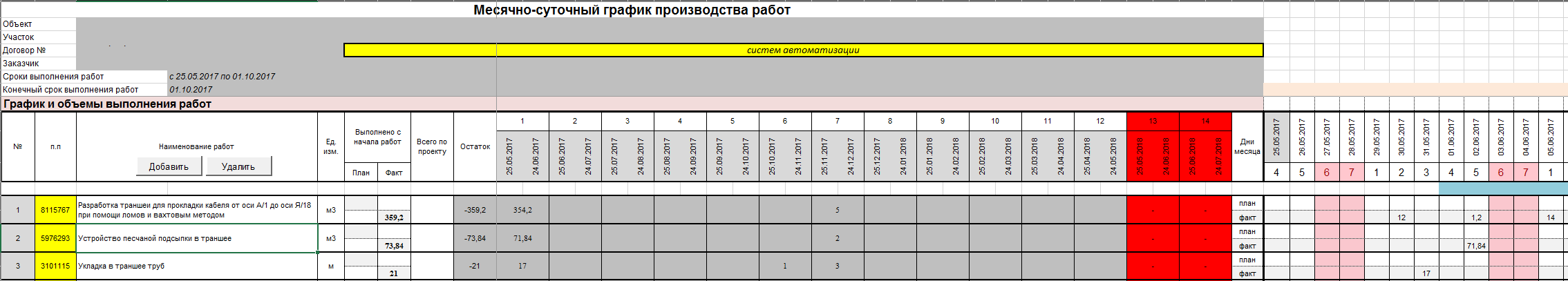
The idea that it is possible to hang a lot of things on it, for example, filling in the General Work Log for part of Section 3 - the name of the work by date, the sequence and the need for the Acts of Examination of the hidden works and not only - took possession of my thoughts. Usually Excel paints dates, depending on the date ranges - the beginning and the end, but not at the construction site !!! At the construction site, in the calendar schedule, volumes are written, and depending on the date from which the volumes of works stand opposite to the name of the works and according to which - the date ranges of the reporting periods are obtained. In the screenshot, gray marks the volumes falling into the systematic reporting periods (1 month). Thus, it turns out that if:

• we detail and draw up the order of works on the project section and write them in turn, then we get the order of works;
• in the calendar, let us designate the reporting periods (gray) and organize the summation of volumes for the reporting periods for each row - we will receive the scope of work for the AOAD and other acts;
• subranges of work for each reporting period can be taken by macro or formula.

Thus, it turns out that with the help of MSG, documentation can be compiled ... And this simplifies both visual perception and visual control of the amount of work.



I hope you were interested. You can try the program at the link



Thanks for attention.