Recognizing scenes in images using deep convolutional neural networks
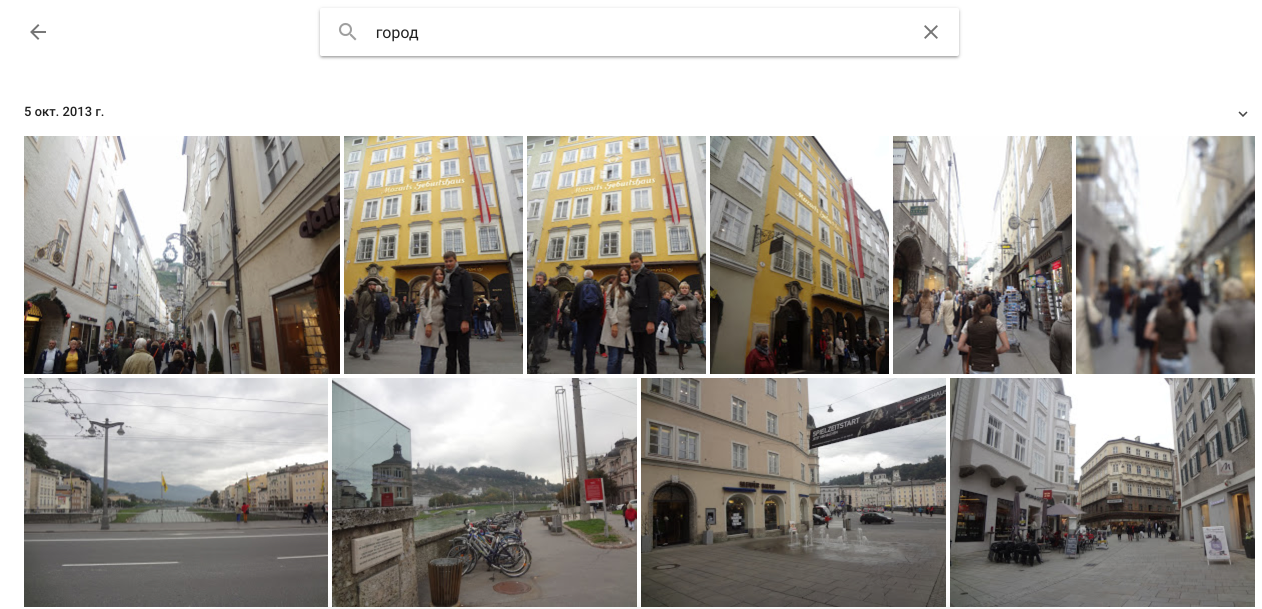
Many products of our company work with images. Some time ago we decided to add to these services a “smart” search through photos, their tagging. Such functionality will be included in the Computer Vision API for further use in the company's products. One of the important ways to tag images is to tag by scenes, when we end up with something like this:
In the Computer Vision community, the object recognition problem has been well studied. One of the main competitions in the field of machine vision is ImageNet , and algorithms (convolutional neural networks since 2012), which won in the object recognition discipline, as a rule, became state-of-the-art. However, the recognition of scenes is studied much less, only from last year this task is included in ImageNet. The main difference between scene recognition (Scene recognition, Place recognition, Place classification) and object recognition is that scenes are more complex entities. For example, in order to determine that the picture shows a kitten, the algorithm needs to detect and recognize one entity - the kitten itself.


')
However, to determine that the restaurant has a picture, you need to find various objects characteristic of it: a table, chairs, counter, kitchen, illuminated menu, visitors, etc. Thus, for the scene recognition it is necessary to determine the context, several objects and interaction with each other.
Modern Computer Vision API can work with scenes. We will see this with examples of the CV API from Google and Microsoft. Both include, among other things, tagging by scene. Examples of the Google CV API:

And Microsoft CV API:

As can be seen from the examples above, both services include scene recognition and find a restaurant in the test picture. Our task was to add similar functionality to our Computer Vision API.
Scene recognition began to actively develop in parallel with the onset of the convolutional neural networks (CNN) boom, that is, around the beginning of the 2010s, when databases began to appear in the public domain. Since our model is a deep CNN, we needed fairly large and diverse datasets to train her. The table shows the main database.
In 2014, the Places base appeared, and in 2016, its second, expanded version of Places2 from MIT. This database can be downloaded in two forms: Places2-Standard and Places2-Challenge. Places2-Standard is a smaller version of Places2-Challenge in which classes are more balanced. The Scene classification competition based on Places2-Challenge was included in ImageNet 2016. The best result in this competition with a top-5 error of 9.01% was shown by the Chinese team Hikvision Research Institute. Examples from the Places2 database are given below, on such data our network was trained.

Learning modern deep CNN even on Places2-Standard takes several days. In order to test and debug various architectures and select the parameters of the model and training in a reasonable time, we decided to take the path that is actively used in Object recognition. There, the models are first tested and debugged on small CIFAR-10 and CIFAR-100 bases, and then the best of them are trained on a large dataset from ImageNet. We cut down the SUN base to 89 classes, 50 thousand images in the training set and 10 thousand in the validation. On the received SUN Reduce dataset, the network learns for about 6-10 hours and gives an idea of its behavior when training on Places2.
In a detailed study of Places2, we decided to get rid of some classes. The reasons for this were the lack of need for these classes in production and too little data, which created a bias in the training set. Examples of such categories are aqueduct, tree house, barndoor. As a result, after cleaning, the base is Places Sift, which consists of 314 classes, the Standard train set includes about 1.5 million images, the Challenge train set includes about 7.5 million images. Also, when studying the categories, it became clear that there were too many of them and they were too detailed to be used in battle. Therefore, we have combined some of them into one, calling this procedure Scene mapping. Here are examples of combining classes:
Scene mapping is applied only when outputting results to the user and only in some tasks where it makes sense. CNN training takes place on the original Places Sift classes. Also in the CV API there is an issue of embedding from the network so that new ones can be retrained based on our model.
Since 2012 (winning the ImageNet team at the University of Toronto, which used CNN AlexNet ), convolutional neural networks have become the de facto state-of-the-art in many areas of Computer Vision and demonstrate significant potential for further progress, therefore in our experiments we considered only this type of models. I will not go into the description of the basics of CNN, some posts are already devoted to this, for example . For a general presentation, the picture below depicts the classic LeNet network from Jan Lekun:
To determine the network architecture, we selected CNN based on the results of ImageNet and Places2 for the last couple of years. The top models in these two competitions can be divided with some degree of conventionality into the Inception family (GoogLeNet, Inception 2-4, Inception-ResNet and their derivatives) and the Residual Networks family (ResNet and various ways to improve it). As a result of our experiments on the recognition of scenes, models from the ResNet family showed themselves best of all, so further narration will be associated with them.
Residual Networks , abbreviated ResNet (can be translated as “residual networks”) appeared at the end of 2015 and won ImageNet 2015. Their inventors are a team from the Asian division of Microsoft Research. They were able to build and successfully train networks of very great depth, that is, with a large number of layers. Comparison of winners of different years in this parameter from the authors:
The main element of ResNet is a Residual block (residual block) with a shortcut connection, through which the data passes unchanged. The res block consists of several convolutional layers with activations that convert the input signal at . A shortcut connection is the same transformation. .

As a result of this design, the Res-block teaches how to input differs from . Therefore, if on some layer the network has already sufficiently well approximated the original function generating the data, then on further layers the optimizer can make the weights close to zero in the Res blocks, and the signal will pass through the shortcut connection almost unchanged. In a sense, it can be said that CNN itself determines its depth.
The most important issue in such a network architecture is the construction of the Res-block. Most of the research and improvements in ResNet are related to this topic. In 2016, an article by the same authors was published , in which they proposed a new way of building the Res-block.

With this approach, it is proposed to make the last activation (ReLU) in the Res-block and move the layers of normalization (batch normalization) and activation before the convolutional layers. This design allows the signal to flow unchanged from one Res block to another. In the article, the authors give a mathematical explanation to the fact that this trick contributes to combating the damped gradient and, therefore, allows you to build networks of very great depth. For example, the authors successfully trained ResNet with 1001 layers.
For our research, the PyTorch framework was chosen because of its flexibility and speed. The comparison of the trained models was carried out according to the measurements of the top-1 and top-5 errors on three tests:
As a result of the experiments, two models were trained: ResNet-50 and ResNet-200. Both networks were connected with ImageNet, as this approach showed a significant advantage in our task before learning from scratch. We compared the trained models on tests with the benchmark model ResNet-152, which was provided by the authors of the base Places2. Top-1 errors:

And top-5 errors:
As can be seen from the graphs, ResNet-200 almost everywhere wins, which, in principle, is not surprising.
Of course, we did not stop at the standard ResNet and, after receiving the results, we continued research on improving the quality of our CNN. A simple increase in the number of layers does not improve. In the article, the authors show that the Residual Network is an ensemble of less deep grids. Below is an illustration of an article on the presentation of ResNet as an ensemble.
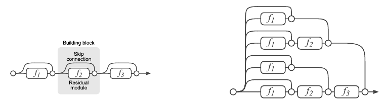
This paper argues that the last Res-blocks make a small contribution to the formation of the final result of the entire network, so a simple increase in the number of blocks does not give the expected result. From these considerations, the idea arose to increase not the depth, but the width of the Residual-block, that is, the number of filters in convolutions.
Launched in 2016, the Wide Residual Network does just that. The author of the work takes the usual ResNet and increases the number of channels in the convolutions in Res-blocks, reaching with a smaller number of quality parameters deeper ResNet. We used the Wide ResNet-50-2 model (WRN-50-2), trained on ImageNet, which is a ResNet-50 with a doubling of channels. The author himself clearly illustrated the difference of the Wide Res block (left) from the classic Res block (right):

WRN-50-2 shows close results for ResNet-200 on ImageNet: 21.9% top-1 errors versus 21.7%. At the same time, the WRN-50-2 is almost twice as fast as the ResNet-200.
For further analysis of the Wide ResNet architecture, let's go back a couple of steps back to the standard Res-block. To increase the efficiency of computations and reduce the number of parameters for large networks, such as ResNet-50/101/152, the authors applied the approach that appeared in the Network In Network model and then was implemented in the Inception model. The idea is to use 1 × 1 convolutions to reduce the number of channels before the more expensive 3 × 3 convolutions, and then restore the original number of channels with another 1 × 1 convolution. The res block with this trick is called a bottleneck. Below is a comparison of the original (left) and bottleneck-blocks (right).
In Wide ResNet, the increase in the number of channels occurs just for “internal” bundles in bottleneck blocks. In the WRN-50-2, the number 64 in the figure on the right increases to 128.
We give a comparison of the trained WRN on our tests. Top-1 errors:
Top 5 errors:
The best model was the WRN-50-2, dubbed with ImageNet and trained on the Places Sift Challenge. It surpassed ResNet-200, while working almost twice as fast. We measured the speed of work on a single GPU Maxwell Titan X, cuDNN 5.0.05 on a batch of 16 images. WRN-50-2 showed 83 ms versus 154 ms for ResNet-200. Such an increase in speed with a close number of parameters can be explained by the “width” of the Res-block and, consequently, by the great possibilities for parallelizing the calculations in it. Training WRN-50-2 took about two weeks.
Here are some examples of how our CNN works using Scene mapping. Examples of successful work (in the format of the prediction and its corresponding speed):

Predicted:
Example of unsuccessful work:

Predicted:
The ResNet family continues to grow. We tried using the last few members of this family to recognize scenes. One of them is the PyramidNet network, which showed promising results on CIFAR-10/100 and on ImageNet. The main idea of this CNN is to gradually increase the number of channels in convolutions, and not sharply several times, as it happens in ordinary ResNet. PyramidNet options:
The authors of the original ResNet are also thinking of expanding the network. They created the ResNeXt model, which offers a “smart” Res-block extension. The basic idea is to decompose the number of channels in the Res block into several parallel streams, for example, 32 blocks with 4 channels = 128 channels instead of the original 64 from the usual Res block (left), as shown in the picture below.
This approach is similar to Inception, but all parallel blocks are the same. With the same complexity of the model as the ResNet, we get an improvement in quality.
Unfortunately, neither PyramidNet nor ResNeXt were able to outperform the WRN-50-2 in our tests and showed similar results.
In the course of the research, we tried several approaches to improving the quality of the network, based on the fact that for each class of scenes there are characteristic objects, and if we learn to distinguish them, then this will help correct the mistakes that the main CNN allows.
The first approach is based on the Class activation map (CAM). Consider the Global average pooling (GAP) layer of our network, followed by the Softmax layer. Denote as the output of the convolution layer before the GAP, - channel number and - spatial coordinates, - weights in the layer after GAP, corresponding to th class. Then:

The basic idea is that instances of one scene should have similar objects as CAM. CAM example for some classes from Places2 after displaying them on the original image:
To implement this approach, we used two networks. Let Network 1 be the new CNN, for example ResNet-50, trained on ImageNet, and Network 2 is our Places Sift WRN-50-2. We tried two types of training. The first algorithm is:
The second algorithm consists of the following steps:
We experimented with both algorithms, but failed to achieve quality improvement.
The next approach we applied to our model is Visual recurrent attention (VRA). The algorithm is rather complicated, and I suggest turning to the article for details, and here I will tell you about its main steps and how we used it in our task. The main idea of VRA is that it “looks” at various image patches, the sequence of which is determined by a recurrent network, and concludes that the entire image is classified according to this sequence. In general, the algorithm looks like this:

In step A of the image several patches are cut in scale with the center at the incoming point . At stage B, these patches, along with the coordinates of the point run through two small networks, resulting in their overall vector representation . It enters the recurrent network. which at each iteration issues a classification decision and the new point of the center of the patches . passes a certain number of steps.
We experimented with VRA, giving it not an image to the input, but a feature map from one of the layers of the WRN-50-2 network after running the input image through it. Our idea was that the Attention mechanism would help to highlight the objects specific to the scene. However, such an algorithm studies for a very long time, and we were not able to raise the quality above 20% in a reasonable time.
In the article that we considered in the section about Wide ResNet, there is an observation that some Res-blocks can be thrown out without a great loss in quality. We conducted experiments to remove several Res-blocks from ResNet-200, however, even with an increase in the speed of its work, the WRN-50-2 remained the best choice for the model.
Now our team continues to experiment in Scene recognition. We train new CNN architectures (mainly from the ResNet family), try other CAM variants, set up Visual Recurrent Attention and try different approaches with more sophisticated image patches.
In this post, we looked at the basic data sets for Scene recognition, different approaches to solving this problem, found out that Wide ResNet still shows the best result, and looked at some methods to improve the model.
In conclusion, I can say that Scene recognition is a necessary, but so far relatively unexplored area of Computer Vision. The task is very interesting, and you can experiment with different approaches that may not be suitable for classic Object recognition (for example, CAM or VRA).
In the Computer Vision community, the object recognition problem has been well studied. One of the main competitions in the field of machine vision is ImageNet , and algorithms (convolutional neural networks since 2012), which won in the object recognition discipline, as a rule, became state-of-the-art. However, the recognition of scenes is studied much less, only from last year this task is included in ImageNet. The main difference between scene recognition (Scene recognition, Place recognition, Place classification) and object recognition is that scenes are more complex entities. For example, in order to determine that the picture shows a kitten, the algorithm needs to detect and recognize one entity - the kitten itself.
')
However, to determine that the restaurant has a picture, you need to find various objects characteristic of it: a table, chairs, counter, kitchen, illuminated menu, visitors, etc. Thus, for the scene recognition it is necessary to determine the context, several objects and interaction with each other.
Modern Computer Vision API can work with scenes. We will see this with examples of the CV API from Google and Microsoft. Both include, among other things, tagging by scene. Examples of the Google CV API:
And Microsoft CV API:
As can be seen from the examples above, both services include scene recognition and find a restaurant in the test picture. Our task was to add similar functionality to our Computer Vision API.
Data
Scene recognition began to actively develop in parallel with the onset of the convolutional neural networks (CNN) boom, that is, around the beginning of the 2010s, when databases began to appear in the public domain. Since our model is a deep CNN, we needed fairly large and diverse datasets to train her. The table shows the main database.
| Base | SUN | LSUN | Places2-Standard | Places2-Challenge |
| Number of categories | 397 | ten | 365 | 365 |
| Number of images | 108 754 | 9 895 373 | 1,803,486 | 8,026,628 |
| Images per class | > 100 | 168 103 - 3 033 042 | 3068 - 5000 | 3068 - 40,000 |
In 2014, the Places base appeared, and in 2016, its second, expanded version of Places2 from MIT. This database can be downloaded in two forms: Places2-Standard and Places2-Challenge. Places2-Standard is a smaller version of Places2-Challenge in which classes are more balanced. The Scene classification competition based on Places2-Challenge was included in ImageNet 2016. The best result in this competition with a top-5 error of 9.01% was shown by the Chinese team Hikvision Research Institute. Examples from the Places2 database are given below, on such data our network was trained.
Learning modern deep CNN even on Places2-Standard takes several days. In order to test and debug various architectures and select the parameters of the model and training in a reasonable time, we decided to take the path that is actively used in Object recognition. There, the models are first tested and debugged on small CIFAR-10 and CIFAR-100 bases, and then the best of them are trained on a large dataset from ImageNet. We cut down the SUN base to 89 classes, 50 thousand images in the training set and 10 thousand in the validation. On the received SUN Reduce dataset, the network learns for about 6-10 hours and gives an idea of its behavior when training on Places2.
In a detailed study of Places2, we decided to get rid of some classes. The reasons for this were the lack of need for these classes in production and too little data, which created a bias in the training set. Examples of such categories are aqueduct, tree house, barndoor. As a result, after cleaning, the base is Places Sift, which consists of 314 classes, the Standard train set includes about 1.5 million images, the Challenge train set includes about 7.5 million images. Also, when studying the categories, it became clear that there were too many of them and they were too detailed to be used in battle. Therefore, we have combined some of them into one, calling this procedure Scene mapping. Here are examples of combining classes:
- bamboo forest, forest broadleaf, forest path, forest road, rainforest -> forest;
- hospital, hospital room, nursery, operating room -> hospital;
- hotel outdoor, hotel room, outdoor, youth hostel -> hotel.
Scene mapping is applied only when outputting results to the user and only in some tasks where it makes sense. CNN training takes place on the original Places Sift classes. Also in the CV API there is an issue of embedding from the network so that new ones can be retrained based on our model.
Approaches, solutions
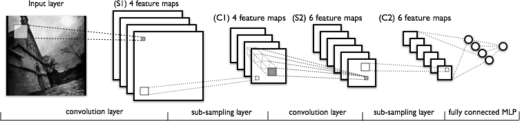
Since 2012 (winning the ImageNet team at the University of Toronto, which used CNN AlexNet ), convolutional neural networks have become the de facto state-of-the-art in many areas of Computer Vision and demonstrate significant potential for further progress, therefore in our experiments we considered only this type of models. I will not go into the description of the basics of CNN, some posts are already devoted to this, for example . For a general presentation, the picture below depicts the classic LeNet network from Jan Lekun:
To determine the network architecture, we selected CNN based on the results of ImageNet and Places2 for the last couple of years. The top models in these two competitions can be divided with some degree of conventionality into the Inception family (GoogLeNet, Inception 2-4, Inception-ResNet and their derivatives) and the Residual Networks family (ResNet and various ways to improve it). As a result of our experiments on the recognition of scenes, models from the ResNet family showed themselves best of all, so further narration will be associated with them.
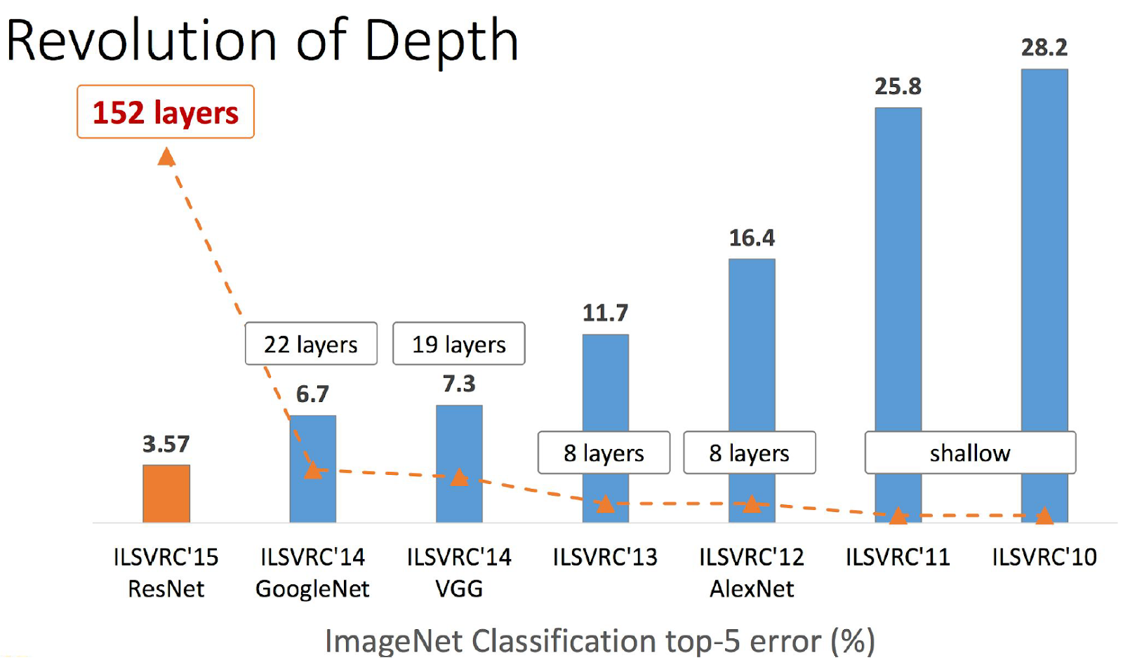
Residual Networks , abbreviated ResNet (can be translated as “residual networks”) appeared at the end of 2015 and won ImageNet 2015. Their inventors are a team from the Asian division of Microsoft Research. They were able to build and successfully train networks of very great depth, that is, with a large number of layers. Comparison of winners of different years in this parameter from the authors:
The main element of ResNet is a Residual block (residual block) with a shortcut connection, through which the data passes unchanged. The res block consists of several convolutional layers with activations that convert the input signal at . A shortcut connection is the same transformation. .
As a result of this design, the Res-block teaches how to input differs from . Therefore, if on some layer the network has already sufficiently well approximated the original function generating the data, then on further layers the optimizer can make the weights close to zero in the Res blocks, and the signal will pass through the shortcut connection almost unchanged. In a sense, it can be said that CNN itself determines its depth.
The most important issue in such a network architecture is the construction of the Res-block. Most of the research and improvements in ResNet are related to this topic. In 2016, an article by the same authors was published , in which they proposed a new way of building the Res-block.
With this approach, it is proposed to make the last activation (ReLU) in the Res-block and move the layers of normalization (batch normalization) and activation before the convolutional layers. This design allows the signal to flow unchanged from one Res block to another. In the article, the authors give a mathematical explanation to the fact that this trick contributes to combating the damped gradient and, therefore, allows you to build networks of very great depth. For example, the authors successfully trained ResNet with 1001 layers.
For our research, the PyTorch framework was chosen because of its flexibility and speed. The comparison of the trained models was carried out according to the measurements of the top-1 and top-5 errors on three tests:
- Places val is a validation set from Places Sift.
- Places val Scene map is a validation set from Places Sift + Scene mapping.
- Manual test - images provided by our colleagues from their clouds, marked up manually. This test is closest to the “combat” use of CNN, but because of the relatively small amount of data, it is less robust.
As a result of the experiments, two models were trained: ResNet-50 and ResNet-200. Both networks were connected with ImageNet, as this approach showed a significant advantage in our task before learning from scratch. We compared the trained models on tests with the benchmark model ResNet-152, which was provided by the authors of the base Places2. Top-1 errors:
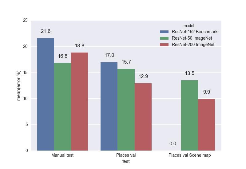
And top-5 errors:
As can be seen from the graphs, ResNet-200 almost everywhere wins, which, in principle, is not surprising.
Wide Residual Network
Of course, we did not stop at the standard ResNet and, after receiving the results, we continued research on improving the quality of our CNN. A simple increase in the number of layers does not improve. In the article, the authors show that the Residual Network is an ensemble of less deep grids. Below is an illustration of an article on the presentation of ResNet as an ensemble.
This paper argues that the last Res-blocks make a small contribution to the formation of the final result of the entire network, so a simple increase in the number of blocks does not give the expected result. From these considerations, the idea arose to increase not the depth, but the width of the Residual-block, that is, the number of filters in convolutions.
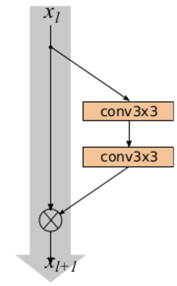
Launched in 2016, the Wide Residual Network does just that. The author of the work takes the usual ResNet and increases the number of channels in the convolutions in Res-blocks, reaching with a smaller number of quality parameters deeper ResNet. We used the Wide ResNet-50-2 model (WRN-50-2), trained on ImageNet, which is a ResNet-50 with a doubling of channels. The author himself clearly illustrated the difference of the Wide Res block (left) from the classic Res block (right):
WRN-50-2 shows close results for ResNet-200 on ImageNet: 21.9% top-1 errors versus 21.7%. At the same time, the WRN-50-2 is almost twice as fast as the ResNet-200.
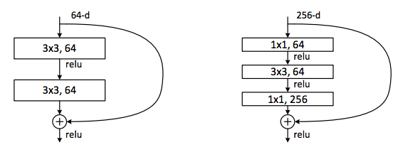
For further analysis of the Wide ResNet architecture, let's go back a couple of steps back to the standard Res-block. To increase the efficiency of computations and reduce the number of parameters for large networks, such as ResNet-50/101/152, the authors applied the approach that appeared in the Network In Network model and then was implemented in the Inception model. The idea is to use 1 × 1 convolutions to reduce the number of channels before the more expensive 3 × 3 convolutions, and then restore the original number of channels with another 1 × 1 convolution. The res block with this trick is called a bottleneck. Below is a comparison of the original (left) and bottleneck-blocks (right).
In Wide ResNet, the increase in the number of channels occurs just for “internal” bundles in bottleneck blocks. In the WRN-50-2, the number 64 in the figure on the right increases to 128.
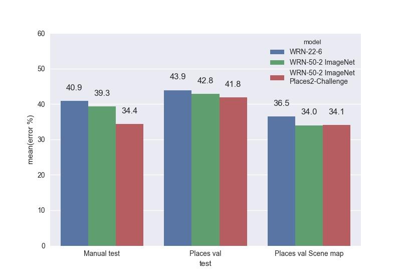
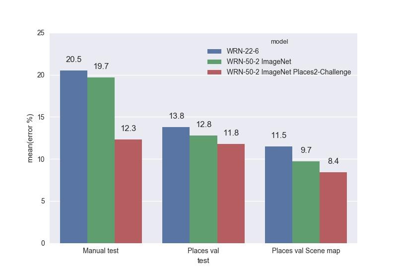
We give a comparison of the trained WRN on our tests. Top-1 errors:
Top 5 errors:
The best model was the WRN-50-2, dubbed with ImageNet and trained on the Places Sift Challenge. It surpassed ResNet-200, while working almost twice as fast. We measured the speed of work on a single GPU Maxwell Titan X, cuDNN 5.0.05 on a batch of 16 images. WRN-50-2 showed 83 ms versus 154 ms for ResNet-200. Such an increase in speed with a close number of parameters can be explained by the “width” of the Res-block and, consequently, by the great possibilities for parallelizing the calculations in it. Training WRN-50-2 took about two weeks.
Work examples
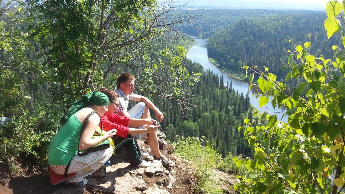
Here are some examples of how our CNN works using Scene mapping. Examples of successful work (in the format of the prediction and its corresponding speed):
| Predicted | Scene mapping |
|
|
| Predicted | Scene mapping |
|
|
Predicted:
- harbor 0,42
- coast 0.13
- cliff 0.12
- promenade 0.07
- ocean 0.04
Example of unsuccessful work:
Predicted:
- palace 0.21
- museum 0.16
- plaza 0.12
- yard 0,1
- church 0,13
Other ResNet
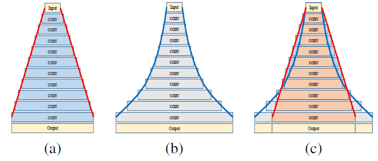
The ResNet family continues to grow. We tried using the last few members of this family to recognize scenes. One of them is the PyramidNet network, which showed promising results on CIFAR-10/100 and on ImageNet. The main idea of this CNN is to gradually increase the number of channels in convolutions, and not sharply several times, as it happens in ordinary ResNet. PyramidNet options:
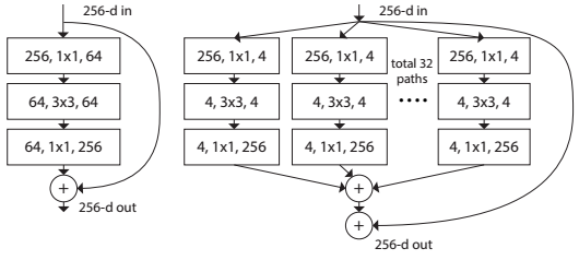
The authors of the original ResNet are also thinking of expanding the network. They created the ResNeXt model, which offers a “smart” Res-block extension. The basic idea is to decompose the number of channels in the Res block into several parallel streams, for example, 32 blocks with 4 channels = 128 channels instead of the original 64 from the usual Res block (left), as shown in the picture below.
This approach is similar to Inception, but all parallel blocks are the same. With the same complexity of the model as the ResNet, we get an improvement in quality.
Unfortunately, neither PyramidNet nor ResNeXt were able to outperform the WRN-50-2 in our tests and showed similar results.
"Creative" approaches to improving CNN
In the course of the research, we tried several approaches to improving the quality of the network, based on the fact that for each class of scenes there are characteristic objects, and if we learn to distinguish them, then this will help correct the mistakes that the main CNN allows.
The first approach is based on the Class activation map (CAM). Consider the Global average pooling (GAP) layer of our network, followed by the Softmax layer. Denote as the output of the convolution layer before the GAP, - channel number and - spatial coordinates, - weights in the layer after GAP, corresponding to th class. Then:
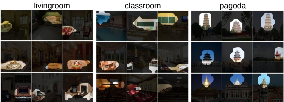
The basic idea is that instances of one scene should have similar objects as CAM. CAM example for some classes from Places2 after displaying them on the original image:
To implement this approach, we used two networks. Let Network 1 be the new CNN, for example ResNet-50, trained on ImageNet, and Network 2 is our Places Sift WRN-50-2. We tried two types of training. The first algorithm is:
- The input image is run through network 2, and a CAM is displayed on it.
- The resulting CAM is run through network 1.
- The result of network 1 is added to the loss function of network 2.
- Network 2 is learning with this new loss feature.
The second algorithm consists of the following steps:
- The input image is run through network 2, and a CAM is displayed on it.
- The resulting CAM is run through network 1.
- Only network 1 is trained.
- When outputting, an ensemble from networks 1 and 2 is used.
We experimented with both algorithms, but failed to achieve quality improvement.
The next approach we applied to our model is Visual recurrent attention (VRA). The algorithm is rather complicated, and I suggest turning to the article for details, and here I will tell you about its main steps and how we used it in our task. The main idea of VRA is that it “looks” at various image patches, the sequence of which is determined by a recurrent network, and concludes that the entire image is classified according to this sequence. In general, the algorithm looks like this:
In step A of the image several patches are cut in scale with the center at the incoming point . At stage B, these patches, along with the coordinates of the point run through two small networks, resulting in their overall vector representation . It enters the recurrent network. which at each iteration issues a classification decision and the new point of the center of the patches . passes a certain number of steps.
We experimented with VRA, giving it not an image to the input, but a feature map from one of the layers of the WRN-50-2 network after running the input image through it. Our idea was that the Attention mechanism would help to highlight the objects specific to the scene. However, such an algorithm studies for a very long time, and we were not able to raise the quality above 20% in a reasonable time.
In the article that we considered in the section about Wide ResNet, there is an observation that some Res-blocks can be thrown out without a great loss in quality. We conducted experiments to remove several Res-blocks from ResNet-200, however, even with an increase in the speed of its work, the WRN-50-2 remained the best choice for the model.
Conclusion
Now our team continues to experiment in Scene recognition. We train new CNN architectures (mainly from the ResNet family), try other CAM variants, set up Visual Recurrent Attention and try different approaches with more sophisticated image patches.
In this post, we looked at the basic data sets for Scene recognition, different approaches to solving this problem, found out that Wide ResNet still shows the best result, and looked at some methods to improve the model.
In conclusion, I can say that Scene recognition is a necessary, but so far relatively unexplored area of Computer Vision. The task is very interesting, and you can experiment with different approaches that may not be suitable for classic Object recognition (for example, CAM or VRA).
Source: https://habr.com/ru/post/359214/
All Articles