Unreal Engine 4 Tutorial: Paint Filter

Over time, the appearance of games is getting better and better. In an era of stunning graphics, it is difficult to make your own game stand out from the rest. One of the ways to make the game more graphically unique is to use non-photorealistic rendering.

Non-realistic rendering includes many rendering techniques. They include cel shading, toon-contours and shading. You can even make the game look like a picture! One way to get this effect is to blur the Kawahara filter.

To implement Kawahara filtering, we will learn the following:
')

• Calculate the mean and variance for several cores.
• Show the average value for the kernel with the lowest variance
• Use the Sobel operator to find the local orientation of a pixel.
• Rotate sampling cores based on pixel local orientation

Note: this tutorial assumes that you are already familiar with the basics of the Unreal Engine. If you only master the Unreal Engine, then study our series of tutorials Unreal Engine for beginners from ten parts.

Since HLSL is used in this tutorial, you should be familiar with it or a language similar to it, for example, C #.

Note: this tutorial is the fourth part of the shader tutorial series:

• Part 1: Cel Shading
• Part 2: Toon-contours
• Part 3: HLSL native shaders
• Part 4: Paint Filter

Getting Started

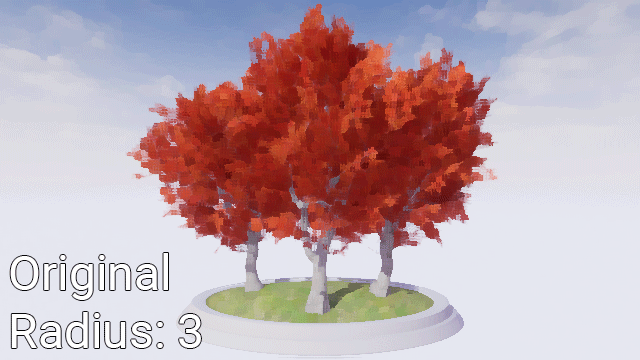
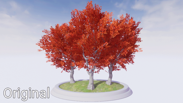
Start by downloading tutorial content . Unzip them, go to PaintFilterStarter and open PaintFilter.uproject . You will see the following scene:


To save time, the scene already has a Post Process Volume with PP_Kuwahara . This is the material (and shader files) that we will modify.


First, let's understand what the Kawahara filter is and how it works.

Filter Kawahara

When shooting photos, you may notice a grainy texture on the image. This is a noise that we absolutely do not need.


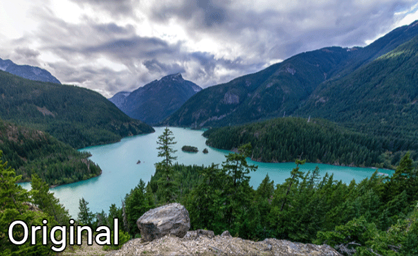
Usually get rid of the noise using a low pass filter, such as blur. Below is a noisy image after applying a box blur to it with a radius of 5.


Most of the noise has disappeared, but all borders have lost their sharpness. That would exist a filter that could smooth the image and preserve the borders of objects!

As you might have guessed, the Kawahara filter meets all these requirements. Let's see how it works.

How Kawahara Filtering Works

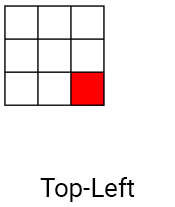
As in convolutions, kernels are used in filtering Kawahars, but four are used instead of one. The cores are arranged in such a way that they overlap in one pixel (in the current). Below is an example of kernels for the Kawahara filter.


First, we calculate the average (average color) for each core. So we erode the core, that is, we smooth the noise.

We also calculate the variance for each core. In fact, it is a measure of how much color varies in the core. For example, a core with similar colors will have a low variance. If the colors are different, then the dispersion of the core will be high .

Note: If you are not familiar with the concept of variance or do not know how to calculate it, then read the article Standard Deviation and Variance on Math is Fun.

Finally, we find the core with the smallest variance and derive its average value. It is thanks to the selection on the basis of the dispersion that the Kawahara filter allows you to maintain boundaries. Let's look at a few examples.

Kawahara filtering examples

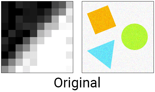
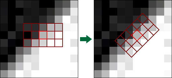
Below is a 10 × 10 image in grayscale. It can be seen that it has a border that goes from the lower left to the upper right corner. You may also notice that in some areas of the image there is noise.


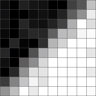
First we select a pixel and determine which core has the smallest variance. Here is the pixel near the border and its associated cores:


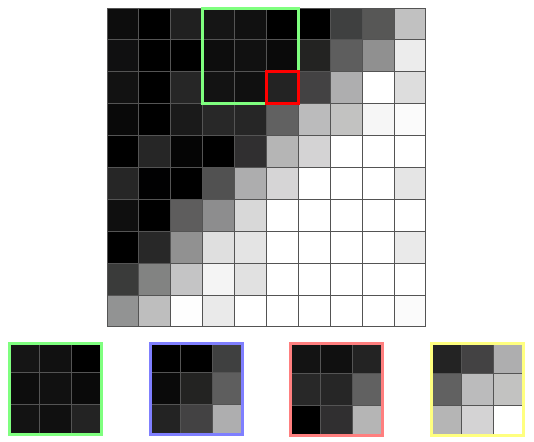
As you can see, the nuclei lying on the border vary greatly in color. This tells us about high dispersion and means that the filter will not select them. Avoiding the choice of kernels lying on the border, the filter eliminates the problem of blurred borders.

For this pixel, the filter will choose the green core, because it is the most homogeneous. The output value will then be the average value for the green core, that is, the color close to black.

Here is another pixel of the border and its core:


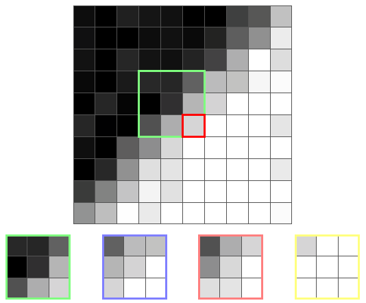
This time the yellow core has the smallest dispersion, because it is the only one that is not on the border. Therefore, the output value will be the average of the yellow core, that is, a color close to white.

Below is a comparison between box blur and Kawahara filtering with a radius of 5.


As you can see, the filtering of Kawahara perfectly copes with smoothing and preserving borders. In our case, the filter even made the border sharper!

Coincidentally, this anti-aliasing function with the preservation of borders can give the image the appearance of a painted picture. Since brush strokes usually have sharp edges and low noise, the Kawahara filter turns out to be a convenient choice for converting realistic images to artistic style.

Here is the result of performing a Kawahara filter for photos with variable size:


Looks pretty nice, right? Let's start creating the Kawahara filter.

Creating a Kawahara filter

In this tutorial, the filter is split into two shader files: Global.usf and Kuwahara.usf . The first file will store the function for calculating the mean and the variance of the kernel. The second file is the input point of the filter, which will call the above function for each core.

First we will create a function to calculate the mean and variance. Open the project folder in the OS and go to the Shaders folder. Then open Global.usf . Inside you will find the GetKernelMeanAndVariance() function.

Before we start creating a function, we need an additional parameter. Change the function signature as follows:

 float4 GetKernelMeanAndVariance(float2 UV, float4 Range) 

To sample the mesh, we need two for : one for horizontal offsets. the second is for vertical. The first two channels of the Range will contain the boundaries of the horizontal loop. The second two will contain the boundaries of the vertical cycle. For example, if we sample the upper left core and the filter has a radius of 2 , then the Range will have the values:

 Range = float4(-2, 0, -2, 0); 

Now it's time to start sampling.

Pixel sampling

First we need to create two for . Add the following code to GetKernelMeanAndVariance() (under variables):

 for (int x = Range.x; x <= Range.y; x++) { for (int y = Range.z; y <= Range.w; y++) { } } 

This will give us all the core offsets. For example, if we sample the upper left core and the filter has a radius of 2 , then the offsets will be in the range from (0, 0) to (-2, -2) .


Now we need to get the pixel color of the sample. Add the following code to the internal for loop:

 float2 Offset = float2(x, y) * TexelSize; float3 PixelColor = SceneTextureLookup(UV + Offset, 14, false).rgb; 

The first line gets the offset of the sample pixel and converts it into UV space. The second line uses the offset to get the color of the sample pixel.

Now we need to calculate the mean and variance.

Calculate the mean and variance

Calculating the average is a fairly simple task. We simply sum up all the colors and divide them by the number of pixels in the sample. For variance, we use the formula below, where x is the color of the sample pixel:


The first thing we need to do is calculate the amounts. To get an average, we just need to add the colors in the variable Mean . To obtain a dispersion, we need to square the color, and then add it to the Variance . Add the following code below:

 Mean += PixelColor; Variance += PixelColor * PixelColor; Samples++; 

Next, add the following after for loops:

 Mean /= Samples; Variance = Variance / Samples - Mean * Mean; float TotalVariance = Variance.r + Variance.g + Variance.b; return float4(Mean.r, Mean.g, Mean.b, TotalVariance); 

The first two lines calculate the mean and variance. However, a problem arises: dispersion is distributed between RGB channels. To solve it, in the third line we summarize the channels to get the total variance.

At the end, the function returns the mean and variance in the form float4 . The average value is in the RGB channels, and the variance is in channel A.

Now that we have a function to calculate the mean and variance, we need to call it for each core. Return to the Shaders folder and open Kuwahara.usf . First we need to create some variables. Replace the code inside with the following:

 float2 UV = GetDefaultSceneTextureUV(Parameters, 14); float4 MeanAndVariance[4]; float4 Range; 

Here is what each variable is used for:

• UV: UV coordinates of the current pixel.
• MeanAndVariance: an array to store the average and variance of each core
• Range: used to store the boundaries of the for loops of the current kernel

Now we need to call for each kernel GetKernelMeanAndVariance() . To do this, add the following:

 Range = float4(-XRadius, 0, -YRadius, 0); MeanAndVariance[0] = GetKernelMeanAndVariance(UV, Range); Range = float4(0, XRadius, -YRadius, 0); MeanAndVariance[1] = GetKernelMeanAndVariance(UV, Range); Range = float4(-XRadius, 0, 0, YRadius); MeanAndVariance[2] = GetKernelMeanAndVariance(UV, Range); Range = float4(0, XRadius, 0, YRadius); MeanAndVariance[3] = GetKernelMeanAndVariance(UV, Range); 

So we get the average and variance of each core in the following order: upper left, upper right, lower left and lower right.

Next, we need to choose a kernel with the smallest variance and derive its average value.

Selection of a kernel with the lowest variance

To select the core with the least variance, add the following code:

 // 1 float3 FinalColor = MeanAndVariance[0].rgb; float MinimumVariance = MeanAndVariance[0].a; // 2 for (int i = 1; i < 4; i++) { if (MeanAndVariance[i].a < MinimumVariance) { FinalColor = MeanAndVariance[i].rgb; MinimumVariance = MeanAndVariance[i].a; } } return FinalColor; 

Here is what each part does:

1. Creates two variables for storing the final color and least variance. Initializes them both with the mean and variance values ​​of the first core.
2. Loops around the remaining three cores. If the dispersion of the current core is lower than the smallest, then its average and dispersion become new FinalColor and MinimumVariance . After executing the cycles, FinalColor is displayed, which will be the average value of the kernel with the least variance.

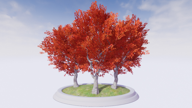
Go back to Unreal and go to Materials \ PostProcess . Open PP_Kuwahara , make no impact changes, and click Apply . Go back to the main editor and look at the results!


It looks pretty good, but if you look closely, you can see that there are strange block areas in the image. I highlighted some of them:


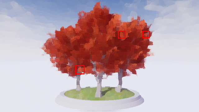
This is a side effect of using core-aligned cores. We can reduce this effect by applying an improved version of the filter, which I call the Kawahara directional filter .

Directional Filter Kawahara

This filter is similar to the original one, but now the cores will be aligned relative to the local orientation of the pixels. Here is an example of a kernel in the directional filter of Kawahara:

Note: since we can represent the core in the form of a matrix, we write the measurements in the form height x width instead of the usual width x height . We will talk more about matrices below.

Here the filter determines the orientation of the pixel so that it is located along the border. Then you can rotate the entire core accordingly.

To calculate the local orientation, the filter performs a convolution pass using the Sobel operator . If the term “Sobel operator” sounds familiar to you, it is because it is a popular border recognition technique. But if this is a method of recognizing boundaries, how can it be used to obtain a local orientation? To answer this question, we need to understand how the Sobel operator works.

How does the operator Sobel

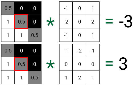
Instead of one core, two are used in the Sobel operator.


Gx gives us a gradient in the horizontal direction. Gy gives us a gradient in the vertical direction. Let’s use this 3 × 3 gray scale image as an example:


First, we perform the convolution of the average pixel for each core.


If each value is plotted on a 2D plane, we will see that the resulting vector points in the same direction as the border.


To find the angle between the vector and the X axis, we substitute the values ​​of the gradients into the arctangent function (atan). After that we can use the resulting angle to rotate the core.

This is how we can use the Sobel operator to get the local orientation of a pixel. Let's try to do it.

Finding a local orientation

Open Global.usf and add the following code inside GetPixelAngle() :

 float GradientX = 0; float GradientY = 0; float SobelX[9] = {-1, -2, -1, 0, 0, 0, 1, 2, 1}; float SobelY[9] = {-1, 0, 1, -2, 0, 2, -1, 0, 1}; int i = 0; 

Note: Notice that the last bracket in GetPixelAngle() missing. This is intentional! If you want to know why to do this, read our HLSL tutorial on shaders .

Here is what each variable is used for:

• GradientX: stores gradient for horizontal direction
• GradientY: stores gradient for vertical direction
• SobelX: the core of the horizontal Sobel operator as an array
• SobelY: the core of the vertical Sobel operator as an array
• i: used to access each element in SobelX and SobelY

Next, we need to perform convolution using SobelX and SobelY cores . Add the following code:

 for (int x = -1; x <= 1; x++) { for (int y = -1; y <= 1; y++) { // 1 float2 Offset = float2(x, y) * TexelSize; float3 PixelColor = SceneTextureLookup(UV + Offset, 14, false).rgb; float PixelValue = dot(PixelColor, float3(0.3,0.59,0.11)); // 2 GradientX += PixelValue * SobelX[i]; GradientY += PixelValue * SobelY[i]; i++; } } 

Here is what happens in each part:

1. The first two lines get the pixel color of the sample. The third line reduces color saturation by converting it to a grayscale value. This simplifies the calculation of the gradients of the image as a whole, instead of obtaining gradients for each color channel.
2. For both cores, multiply the pixel value in shades of gray by the corresponding core element. Then we add the result to the corresponding gradient variable. Then increment i occurs so that it contains the index of the next kernel element.

To get the angle, we use the atan() function and substitute our gradient values. Under the for loops, add the following code:

 return atan(GradientY / GradientX); 

Now that we have a function for obtaining the pixel angle, we need to somehow apply it to rotate the core. We can do this with a matrix .

What is a matrix?

A matrix is ​​a two-dimensional array of numbers. For example, here’s a 2 × 3 matrix (with two rows and three columns):


By itself, the matrix does not look particularly interesting. But the true power of matrices is manifested when we multiply it with a vector. This allows us to perform actions such as rotation and scaling (depending on the type of matrix). But how do we create a matrix for the rotation?

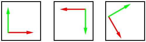
In the coordinate system, we have a vector for each dimension. These are the basic vectors defining the positive directions of the axes.

Below are some examples of different basis vectors for a two-dimensional coordinate system. The red arrow shows the positive direction in X. The green arrow indicates the positive direction in Y.


To rotate a vector, we can use these basis vectors to construct a rotation matrix . It is simply a matrix containing the positions of the basis vectors after rotation. For example, imagine that we have a vector (orange arrow) in coordinates (1, 1) .


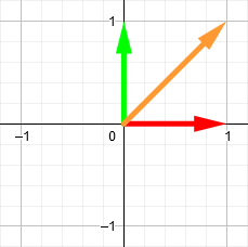
Suppose we want to rotate it 90 degrees clockwise. First, we rotate the basis vectors by the same amount.


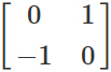
Then we build a 2 × 2 matrix, applying the new positions of the basis vectors. The first column is the position of the red arrow, and the second is the position of the green arrow. This is our rotation matrix.


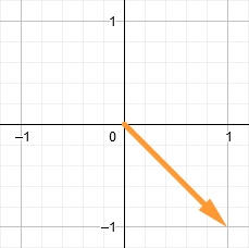
Finally, we perform matrix multiplication using an orange vector and a rotation matrix. The result will be the new position of the orange vector.

Note: you do not need to know how matrix multiplication is performed, because HLSL has a built-in function for this. But if you want to know, then study the article How to Multiply Matrices on Math is Fun.

Is not that great? But even better, we can use the matrix shown above to rotate any 2D vector 90 degrees clockwise. If we talk about our filter, it means that we need only once to create a rotation matrix for each pixel and use it for the entire core.

Now it's time to rotate the core using the rotation matrix.

Core rotation

First we need to change GetKernelMeanAndVariance() to get a 2 × 2 matrix. This is necessary because we will create a rotation matrix in Kuwahara.usf and transmit it. Change the GetKernelMeanAndVariance() signature as follows:

 float4 GetKernelMeanAndVariance(float2 UV, float4 Range, float2x2 RotationMatrix) 

Next, replace the first line of the inner for loop with the following code:

 float2 Offset = mul(float2(x, y) * TexelSize, RotationMatrix); 

mul() will perform matrix multiplication using offset and RotationMatrix . So we will rotate the offset around the current pixel.

Next, we need to create a rotation matrix.

Creating a rotation matrix

To create the rotation matrix, we apply the sine and cosine functions as follows:


Close Global.usf and open Kuwahara.usf . Then add the following below the list of variables:

 float Angle = GetPixelAngle(UV); float2x2 RotationMatrix = float2x2(cos(Angle), -sin(Angle), sin(Angle), cos(Angle)); 

The first line calculates the angle of the current pixel. The second line creates a rotation matrix using an angle.

Finally, we need to pass for each RotationMatrix core. Change each call to GetKernelMeanAndVariance() as follows:

 GetKernelMeanAndVariance(UV, Range, RotationMatrix) 

And on this we have completed the creation of the directional filter Kawahara! Close Kuwahara.usf and return to PP_Kuwahara . Make no impact changes, click Apply and close it.

The image below shows a comparison of the conventional and directional Kawahara filters. Note that the directional filter does not create blockiness.

Note: You can use PPI_Kuwahara to resize the filter. I recommend changing the filter size so that the radius of X is greater than the radius of Y. This will increase the size of the core along the border and will help in creating directivity.

Where to go next?

Download the finished project at the link .

If you want to know more about the Kawahara filter, then you can read the article about the Kawahara anisotropic filtering . In fact, the Kawahara directional filter is a simplified version of the filter presented in this article.

I recommend that you experiment with the matrices in order to use them to create new effects. For example, you can use a combination of rotation and blur matrices to create a radial or circular blur. If you want to know more about matrices and how they work, then learn the 3Blue1Brown video series Essence of Linear Algebra .