Vinyl Data Storage

In 2016, I spoke at Highload with a report about Vinyl , a disk data storage engine in Tarantool. Since then, we have added many new features, but the storage of data on disk is such a voluminous topic that the fundamentals discussed in this article have not changed at all.
Content (so that it is convenient to navigate):
')
- Why did we write a new engine?
- Algorithm
- LSM benefits
- LSM Disadvantages And Their Elimination
- Advanced Vinyl Features
- Conclusion
Why did we write a new engine?
As you know, Tarantool is a transactional, persistent DBMS that stores 100% of data in RAM. The main advantages of storing in RAM are speed and ease of use: the database does not need to be tipped, however, the performance remains consistently high.
A few years ago, we were puzzled by the expansion of the product with the classic storage technology - as in conventional DBMS, when only the data cache is stored in RAM, and the main volume is pushed out to disk. We decided that the storage engine could be selected independently for each table, as implemented in MySQL, but the transaction support will be implemented from the very beginning.
The first question to answer was: to create your own engine or use an existing library? There are ready libraries in the open source community that could be used. At the time of the selection, the RocksDB library was most actively developed, which has by now become one of the most popular. But there were also a number of lesser-known libraries: WiredTiger, ForestDB, NestDB, LMDB.
Nevertheless, having looked at the source code of the existing libraries and having weighed all the pros and cons, we decided to write our own.
All third-party libraries that exist today assume that requests for data can come from multiple operating system threads, and contain complex synchronization primitives to control simultaneous access to data. And if they are embedded in our architecture, then users will be forced to bear the costs of multi-threaded applications without getting anything in return.
The fact is that at the core of Tarantool is actor based architecture. Our approach to processing transactions in a dedicated thread eliminates unnecessary locks, interprocess communication, and other overhead, consuming up to 80% of the processor time of multi-threaded DBMS.
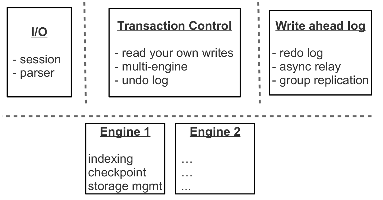
The Tarantool process consists of a fixed number of role-playing streams.
And if you initially design a storage subsystem with an eye on cooperative multitasking, you can not only significantly speed up the work, but also implement optimizations that are too complex for multithreaded engines. In general, integrating a third-party solution in Tarantool, we would not get the best result.
Algorithm
Having abandoned the idea of embedding existing libraries, it was necessary to decide on the basis of which architecture to build one’s own. Today there are two generations of disk storage solutions: using varieties of B-trees and new ones built on the basis of LSM-trees (Log Structured Merge Tree). For example, MySQL, PostgreSQL, Oracle use B-trees, and Cassandra, MongoDB, CockroachDB already use LSM.
It is considered that B-trees are more efficient for reading, and LSM-trees for writing. However, with the proliferation of SSDs that have several times higher read performance than write performance, the advantages of LSM have become apparent for most scenarios.
Before we figure out how LSM trees are organized in Tarantool, let's see how they work. To do this, we will analyze the device of the usual B-tree and the problems associated with it.
“B” in the name of B-tree means Block, that is, it is a balanced tree consisting of blocks. The block contains a sorted list of items, that is, key + value pairs. Omit the questions of filling the tree, balancing, splitting and merging blocks, you can read the details in Wikipedia. As a result, we get a container sorted in ascending order of a key, the minimum element of which is stored in the leftmost node, and the maximum one - in the rightmost one. Let us analyze how the B-tree searches and updates data.
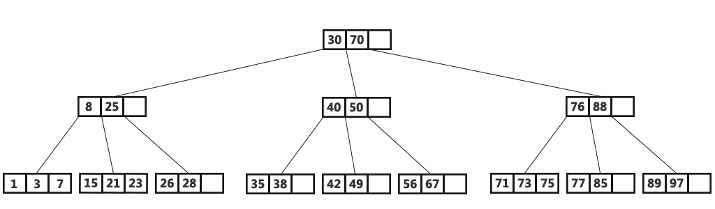
Classic B-tree
If you need to find an element or check its availability, we begin the search, as usual, from the top. If the key is found in the root block, the search ends; otherwise, we move to the block with the largest smaller key, that is, to the rightmost block, in which there are still less than the required items (elements at all levels are arranged in ascending order). In case the element is not found there, we again go to the level below. In the end we will be in one of the leaves and, perhaps, we will find the desired element. It is assumed that tree blocks are stored on disk and read into whole RAM, that is, in one search, the algorithm reads log B (N) blocks, where N is the number of elements in the tree. Record in the simplest and most mass case is carried out in a similar way: we find the block containing the required element and update (insert) the value in it.
To visualize this structure, let's take a tree with 100,000,000 nodes and assume that the block size is 4096 bytes and the size of the element is 100 bytes. In the block, taking into account the overhead, it will be possible to place up to 40 elements. The tree will have about 2,570,000 blocks, five levels, while the first four will occupy about 256 MB, and the last - about 10 GB. Obviously, on any modern computer, all levels except the last will successfully fall into the cache of the file system, and virtually any read operation will require no more than one I / O operation.
The situation looks much less rosy when you change the point of view. Suppose we update one element of the tree. Since tree operations work through reading and writing blocks, we are forced to read 1 block into memory, change 100 bytes from 4096, and write new block to disk. Thus, we had to record 40 times more than the actual amount of changed data! Taking into account that the internal block size in SSD disks can be 64KB and more, and not any element change changes it entirely, the amount of “parasitic” disk load can be even higher.
The phenomenon of “parasitic” readings in literature and blogs dedicated to disk storage is called read amplification, and the phenomenon of parasitic writing is called write amplification. Formally, the amplification factor, that is, the multiplication factor, is calculated as the ratio of the size of the actually read (or recorded) data to the actually needed (or modified) size. In our example with a B-tree, the ratio will be around 40 for both reading and writing.
The amount of parasitic I / O operations when updating data is one of the main problems that LSM-trees solve. Let's take a look at how this works.
The key difference between LSM trees and classic B-trees is that LSM does not store data, that is, keys and values, but data operations: inserts and deletes.
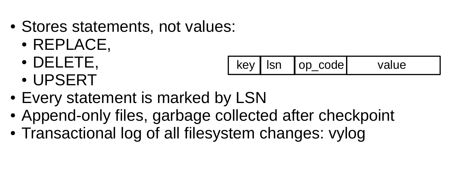
For example, the element for the insert operation, in addition to the key and value, contains an additional byte with the operation code — denoted as REPLACE in the illustration. Deletion contains the key of the item (there is no need to store the value) and the DELETE opcode. Also, each LSM element contains a sequence number of a log sequence number (LSN) operation — a value of a monotonically increasing sequence that uniquely identifies each operation. Thus, the entire tree is ordered first in ascending order of the key, and within the same key in descending order of LSN.

Device level
Filling LSM tree
Unlike the B-tree, which is completely stored on disk and can be partially cached in RAM, in the LSM tree the separation between memory and disk is clearly present from the very beginning. In this case, the problem of data integrity, located in volatile memory, is taken out of the brackets of the storage algorithm: it can be solved in different ways, for example, by logging changes.
The part of the tree located in RAM is called L0 (level zero). The amount of RAM is limited, so a fixed area is allocated for L0. In the Tarantool configuration, for example, the size of L0 is given by the vinyl_memory option. At the beginning, when the tree contains no elements, the operations are written in L0. Let me remind you that the elements in the tree are ordered by the ascending key, and then by descending LSN, so in the case of inserting a new value by this key, it is easy to detect and delete the previous one. Presented L0 can be any container that preserves the ordering of elements. For example, Tarantool uses to store L0 B + * - tree, which I talked about in my blog . The search and insert operations in L0 are standard operations of the data structure used to represent L0, and we will not consider them in detail.
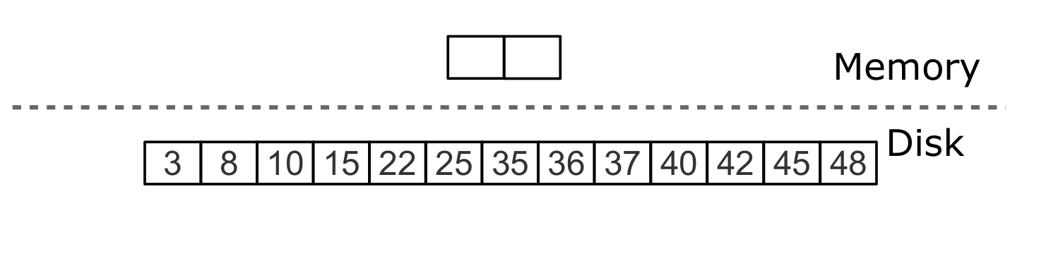
Sooner or later the number of elements in the tree will exceed the size of L0. Then L0 is written to a file on disk and released for new inserts. This operation is called dump.
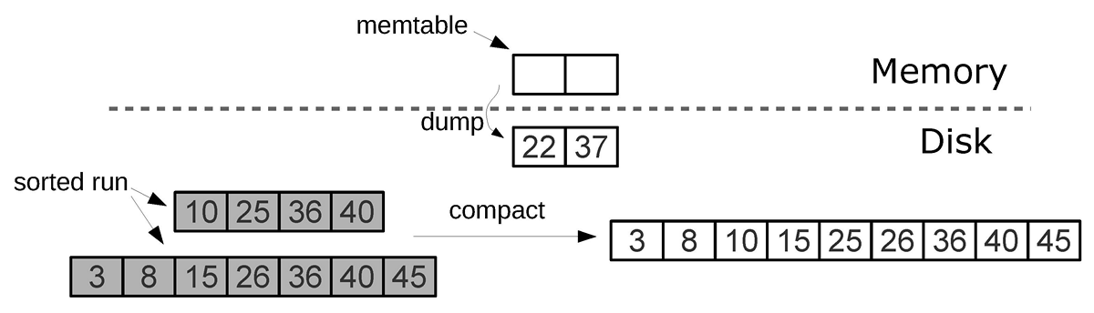
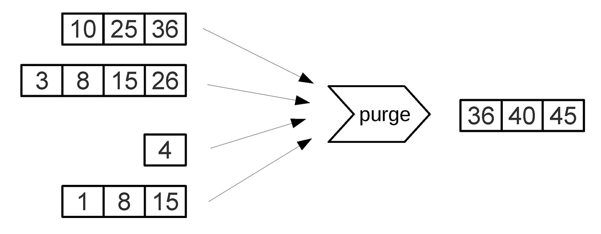
All dumps on a disk form a sequence ordered by LSN: the LSN ranges in the files do not intersect, and closer to the beginning of the sequence are files with newer operations. Imagine these files in the form of a pyramid, placing the new files at the top, and the old at the bottom. As new files appear, the height of the pyramid grows. In this case, more recent files may contain delete or replace operations for already existing keys. To delete old data, you need to collect garbage (this process is sometimes called merge, which can be translated as a merge, and sometimes compaction, which is more correctly translated as garbage collection), combining several old files into a new one. If during the merge we encounter two versions of the same key, then it is enough to leave only a newer version, and if after inserting the key it was deleted, then both operations can be excluded from the result.
A key factor in the effectiveness of the LSM tree is at what point and for which files is the merge. Imagine that a tree stores a monotone sequence of the form 1, 2, 3 ... as keys, and there are no delete operations. In this case, the merging will be useless - all elements are already sorted, the tree does not contain garbage and you can uniquely determine in which file each key is located. In contrast, if a tree contains many deletes, a merge will free up disk space. But even if there are no deletions, and the key ranges in different files overlap strongly, a merge can speed up the search, as it will reduce the number of files to view. In this case, it may make sense to perform a merge after each dump. However, such a merge will result in overwriting of all data on the disk, so if there are few readings, then it is better to do merges less frequently.
In order to optimally configure the LSM tree under any of the above scenarios, LSM organizes all the files into a pyramid: the newer the data operations, the higher they are in the pyramid. In this case, two or more adjacent files in the pyramid participate in the merge; whenever possible, files of approximately the same size are selected.
All adjacent files of approximately the same size make up the level of the tree on the disk. The ratio of file sizes at levels determines the proportions of the pyramid, which allows you to optimize the tree for intensive inserts or intensive reads.
Assume that the L0 size is 100 MB, and the step (ratio) of the file sizes at each LSM level (variable vinyl_run_size_ratio) is 5, while at each level there can be no more than 2 files (variable vinyl_run_count_per_level). After the first three dumps, 3 files of 100 MB each will appear on the disk, these files form the L1 level. Since 3> 2, the file merging (compaction) will start, resulting in a new file with a size of 300 MB, and the old ones will be deleted. After another 2 dumps, the merge will start again, this time with 100, 100 and 300 MB files, as a result, the 500 MB file will be moved to the L2 level (the ratio of the level sizes is 5), and the L1 level will “empty”. It will take another 10 dumps, and we will get 3 files of 500 MB at the L2 level, as a result of which one file of 1500 MB will be created. After another 10 dumps, during which we will merge 3 files of 100 MB each 2 times and merge files of 100, 100 and 300 MB 2 times, we will get two more files at the L2 level of 500 MB, and as a result the merger will start L2 level, which will create the first file in 2500 MB. This file, due to its size, will move to the L3 level.
The process can go on indefinitely, and if there are many deletions in the LSM tree workflow, the merged file can move not only down the pyramid, but also up, since it will be less than the original merge files. In other words, it is logical to track the file belonging to a level logically - based on the file size and the minimum and maximum LSN among all operations stored in it.
Controlling the shape of the LSM tree
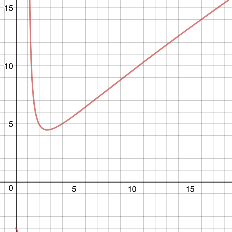
If the number of files to search should be reduced, then the ratio of file sizes at different levels increases, and, as a result, the number of levels decreases. If, on the contrary, it is necessary to reduce the costs caused by compaction, then the ratio of the size of the levels decreases, the pyramid becomes higher, and compaction, although it is performed more often, but works on average with smaller files, due to which it performs less work in total. In general, for given N — the total size of all elements of the tree, L0 — the level zero size, and x — the level size ratio (level_size_ratio), write amplification in the LSM tree is described by the formula log x (N / L0) × x, or x × ln (N / C0) / ln (x), whose graph for x with N / C0 = 40 (disk: memory ratio) looks like this:
Read amplification is proportional to the number of levels. The cost of searching at each level does not exceed the cost of searching in the B-tree. For our “canonical” tree of 100,000,000 elements, 256 MB of RAM and the standard values of vinyl_level_size_ratio = 3.5 and run_count_per_level = 2, we get write amplification factor of about 13. At the same time, read amplification can go up to 150. Let's see why read amplification will be so big.
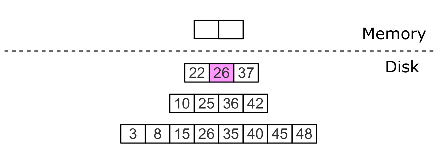
Search
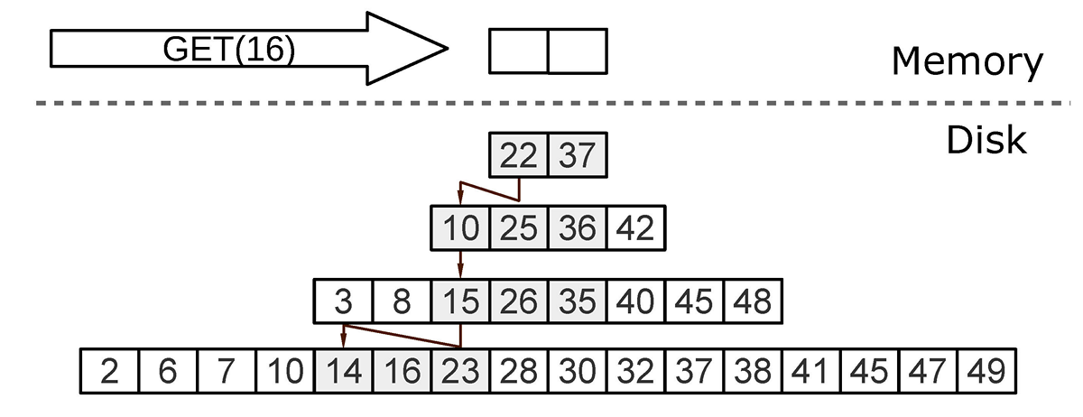
When searching in the LSM tree, we need to find not the element itself, but the last operation with it. If this is a delete operation, the item is not in the tree. If this is an insert operation, then the top item in the LSM pyramid corresponds to the search element, and the search can be stopped when the key first matches. In the worst case, the value in the tree was initially absent. Then the search is forced to sequentially iterate through all levels of the tree, starting with L0.
Unfortunately, in practice, this worst case is quite common. For example, when inserting into a tree for a primary or unique key, you must ensure that there are no duplicates. To speed up the search for "non-existent" values in LSM, a probabilistic data structure is used - the Bloom filter. We will talk about them in more detail in the section on the internal arrangement of Vinyl.
Search by range
If, when searching by one key, the algorithm ends after the first match, then to search for all values in the range, for example, all users with the last name "Ivanov", it is necessary to look through all levels of the tree.
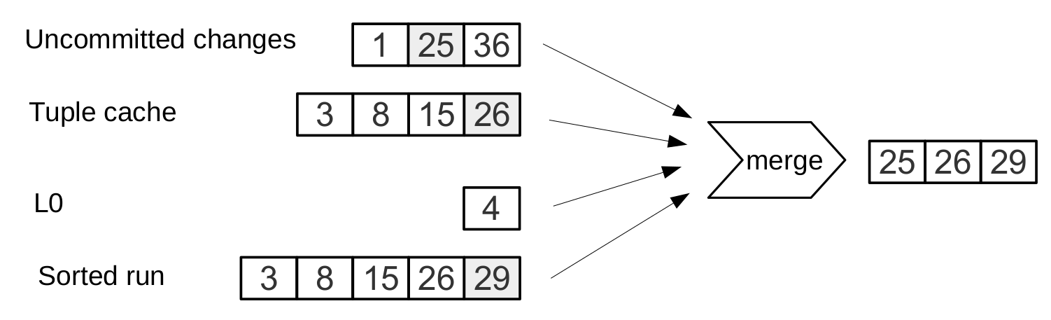
Search by range [24,30)
In this case, the formation of the desired range occurs in the same way as when merging files: from all sources a key with the maximum LSN is selected, the remaining operations on this key are discarded, and the search position is shifted to the next key.
Deletion
Why even keep the deletion? And why does this not lead to tree overflow, for example, in the script for i = 1,10000000 put (i) delete (i) end?
The role of deletion operations during the search is to signal the absence of the desired value, and when merging, to clear the tree of “junk” entries with an older LSN.
As long as the data is stored only in RAM, there is no need to store the deletion. There is also no need to save deletes after a merge, if it affects, including the lowest level of the tree - it contains the data of the oldest dump. Indeed, the absence of a value in the last level means that it is absent from the tree.

Delete, step 1: insert into L0
Uninstall, step 2: tombstone passes through intermediate levels
Delete, step 3: when major compaction, tombstone is removed from the tree.
If we know that deletion immediately follows the insertion of a unique value, and this is a common case when the value in the secondary index changes, then the deletion operation can be filtered out at the merging of intermediate levels. This optimization is implemented in Vinyl.
LSM benefits
In addition to reducing the write amplification, the approach with periodic unloading (dump) of the L0 level and merging (compaction) of the L1-Lk levels has several advantages over the recording approach used in the B-tree:
- Dump and compaction write relatively large files: the typical size of L0 is 50-100 MB, which is thousands of times larger than the size of a B-tree block.
- Large size allows you to effectively compress data before recording. In Tarantool, the compression is automatic, which makes it possible to further reduce write amplification.
- , /.
- , . , , . .
- , multi-version concurrency control.
LSM
B- : log B (N). LSM , . , L0 , L1, L2 .. L0, . , , B-. , . , Tarantool.
LSM L0. , , L0, ?
L0 : . L0 , Tarantool .
, L0 256 M. 10 /. L0 26 . 10 000 , — 100 . 26 M , L0 230 M.
Tarantool , . L0 . , (vinyl_timeout), 60 . , (2 ) vinyl_write_threads. 2 dump compaction, .
Tarantool , . append-only — , compaction .
L0 , : L0 — . L0 , . , , . : L0 , .
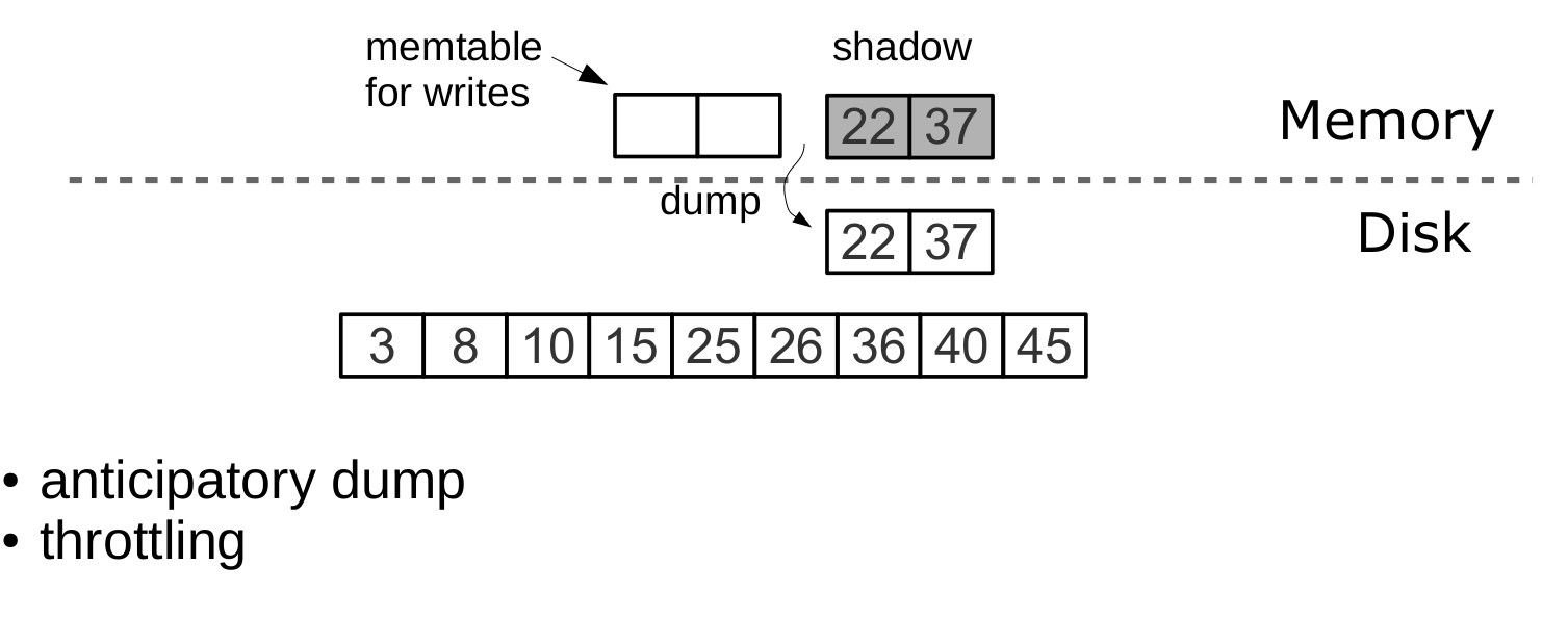
Dump «shadow» L0,
— LSM-. : , . , append-only LSM- .
B- , , . , MySQL PostgreSQL. LSM :
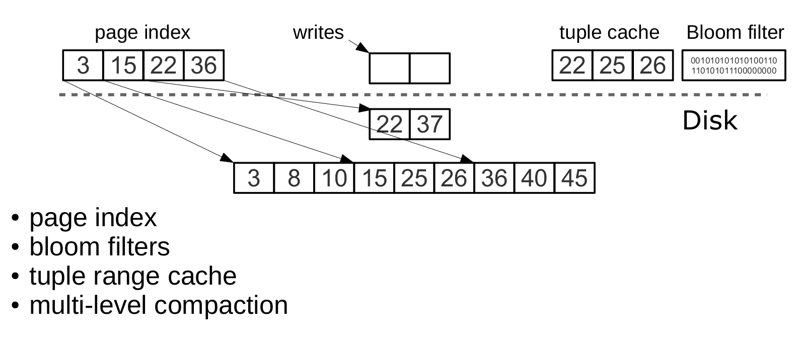
. vinyl_page_size, . , vinyl_page_size — , . . zstd Facebook. page index — , . page index . .index- . .run- ( Vinyl , ). , . , vinyl_read_threads.
Tarantool . , .run- .xlog-, . , .
Bloom-
Although page index allows you to reduce the number of pages viewed when searching in a single file, it does not eliminate the need to search in all levels of the tree. There is an important special case when it is necessary to check the absence of data, and then viewing all levels is inevitable: insertion into a unique index. If the data already exists, then insertion into a unique index should complete with an error. The only way to return an error before completing a transaction in the LSM tree is to search before insertion. Such readings in a DBMS form a whole class called “hidden” or “parasitic” readings.
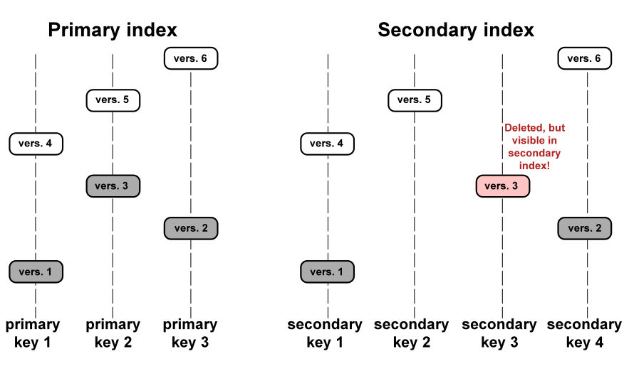
Another operation that leads to hidden reads is an update of the value for which the secondary index is built. Secondary keys are regular LSM trees in which data is stored in a different order. Most often, in order not to store all data in all indexes, the value corresponding to a given key is stored entirely in the primary index (any index that stores both the key and the value is called covering or clustered), and only fields on the secondary index are stored. which built the secondary index, and the values of the fields participating in the primary index. Then, for any change in the value for which the secondary key is built, it is necessary to first remove the old key from the secondary index, and only then insert the new one. The old value during the update is unknown - that’s what you need to read from the primary key “under the hood”.
For example:
update t1 set city='Moscow' where id=1To reduce the number of reads from the disk, especially for non-existent values, almost all LSM-trees use probabilistic data structures. Tarantool is no exception. Classic Bloom filter (Bloom filter) is a set of several (usually 3-5) bit arrays. When writing, several hash functions are calculated for each key, and a bit corresponding to the hash value is set in each array. During hashing, collisions may occur, so some bits can be stamped twice. Of interest are the bits that were not stamped after recording all the keys. The search also calculates selected hash functions. If at least one of the bit arrays does not have a bit, then there is no value in the file. The probability of triggering a bloom filter is determined by the Bayes theorem — each hash function is an independent random variable, so the probability that a collision will occur in all bitmaps at the same time is very small.
A key advantage of implementing Tarantool's Bloom filters is the ease of setup. The only configuration parameter that can be changed independently for each index is called bloom_fpr (fpr is short for false positive ratio), which is 0.05 by default, or 5%. Based on this parameter, Tarantool automatically builds Bloom filters of optimal size for searching in both partial and full keys. The Bloom filters themselves are stored with page index in the .index file and are cached in RAM.
Caching
Many are accustomed to considering caching a panacea for all performance problems. In any incomprehensible situation, add a cache. In Vinyl, we look at the cache rather as a means of reducing the overall load on the disk, and, as a result, obtaining a more predictable response time to queries that did not fall into the cache. Vinyl implements a kind of cache that is unique for transactional systems: range tuple cache. Unlike RocksDB, for example, or MySQL, this cache does not store pages, but ready-made ranges of index values, after reading them from disk and merging all levels. This allows you to use the cache for queries both on a single key and on a range of keys. Since only hot data is stored in the cache, and not, for example, pages (only a part of data can be claimed on a page), RAM is used most optimally. The cache size is set by the vinyl_cache configuration variable.
Garbage collection management
Perhaps, having reached this place, you have already begun to lose focus and need a well-deserved dose of dopamine. It's time to take a break, because in order to deal with the rest, it will take serious efforts.
In a Vinyl device, a single LSM tree is just a puzzle piece. Vinyl creates and maintains several LSM-trees, even for one table (space) - one tree for each index. But even a single index can consist of dozens of LSM-trees. Let's try to figure out why.
Consider our standard example: 100,000,000 entries of 100 bytes each. After some time, at the lowest LSM level, we may have a 10 GB file. During the merge of the last level, we will create a temporary file, which will also occupy about 10 GB. Data at intermediate levels also occupy space - a tree can store several operations using the same key. In total, we may need up to 30 GB of free space to store 10 GB of usable data: 10 GB for the last level, 10 GB for a temporary file and 10 GB for everything else. And if the data is not 1 GB, but 1 TB? Requiring that the amount of free disk space is always several times larger than the amount of useful data is not economically viable, and creating a file in 1TB can take dozens of hours. In case of any accident or system restart, the operation will have to be restarted.
Consider another problem. Imagine that the primary key of a tree is a monotonous sequence, for example, a time series. In this case, the main inserts will fall on the right side of the key range. It makes no sense to re-merge just to add a few million more records to the tail of an already huge file.
And if inserts occur, basically, in one part of a range of keys, and readings - from other part? How in this case to optimize the shape of the tree? If it is too high, the reading will suffer, too low - the record.
Tarantool “factorizes” the problem, creating not one, but many LSM-trees for each index. The approximate size of each subtree is given by the variable vinyl_range_size and defaults to 1 GB, and the subtree itself is called range.
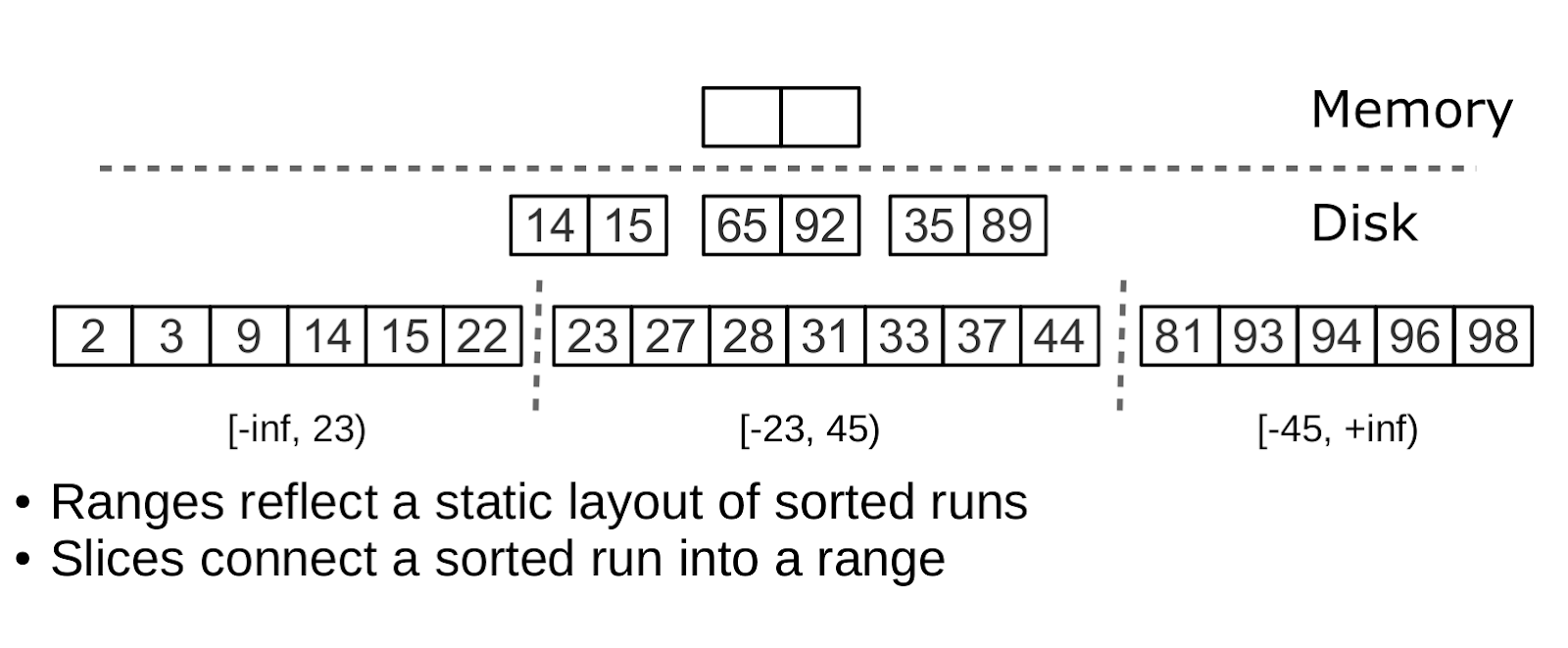
Factorizing large LSM trees using rankings
Initially, while there are few elements in the index, it consists of a single range. As you fill, the total volume may exceed vinyl_range_size. In this case, the split operation is performed - dividing the tree into two equal parts. The separation takes place according to the middle element of the range of keys stored in the tree. For example, if the tree initially stores the full range -inf ... + inf, then after splitting the middle key X we will get two subtrees: one will store all keys from -inf to X, the other - from X to + inf. Thus, when inserting or reading, we definitely know which subtree to refer to. If there were deletions in the tree and each of the adjacent ranges is “lost”, the reverse operation is performed - coalesce. It combines two adjacent trees into one.
Split and coalesce do not lead to merging, creating new files and other heavy operations. An LSM tree is just a collection of files. In Vinyl, we implemented a special metadata journal that makes it easy to track which file belongs to which subtree or subtrees. The log has the .vylog permission, is compatible with the format of the .xlog file, and, like the .xlog file, is automatically rotated with each checkpoint. To avoid re-creating files with split or coalesce, we introduced an intermediate entity - slice. This is a link to the file, indicating the range of key values that is stored exclusively in the metadata log. When the number of links to the file becomes zero, the file is deleted. And when it is necessary to produce split or coalesce, Tarantool creates slice-objects for each new tree, removes old slice objects, and writes these operations to the metadata log. Literally, the metadata log stores records like <tree id, slice id> or <slice id, file id, min, max>.
Thus, the direct hard work of splitting a tree into two subtrees is postponed until compaction and is performed automatically.
A huge advantage of the approach with the division of the entire range of keys into subranges (ranges) is the ability to independently control the size of L0, as well as the dump and compaction process for each subtree. As a result, these processes are manageable and predictable. Having a separate metadata log also simplifies the implementation of operations such as truncate and drop — in Vinyl, they are processed instantly because they work exclusively with the metadata log, and garbage collection is performed in the background.
Advanced Vinyl Features
Upsert
Earlier, I wrote only about two operations that the LSM tree stores: delete and replace. Let's look at how everyone else is represented. Insert can be represented using replace, you just need to make sure in the absence of an element with the same key. To update we also have to pre-read the old value from the tree, so this operation is easier to write to the tree as replace - this will speed up future readings on this key. In addition, update should return a new value, so that hidden readings can not be avoided.
In B-trees, hidden readings cost almost nothing: in order to update a block, in any case, it must be read from the disk. For LSM trees, the idea of creating a special update operation that would not lead to hidden reads looks very tempting.
Such an operation should contain both a default value that needs to be inserted if there is no data on the key yet, and a list of update operations to be performed if the value exists. At the stage of transaction execution, Tarantool only saves the entire operation in the LSM tree, and “performs” it only during the merge.
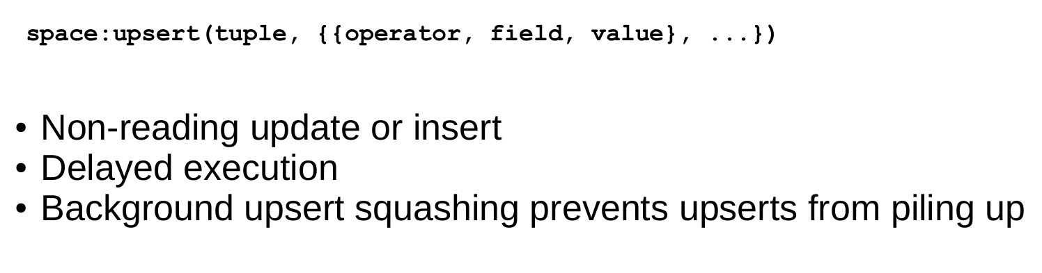
Upsert operation
Unfortunately, if you postpone the execution of the operation at the merge stage, there are no good options for error handling. Therefore, Tarantool seeks to validate the upsert operations as much as possible before writing to the tree, but some checks can be performed only with old data on hand. For example, if update adds a number to a string or removes a nonexistent field.
An operation with similar semantics is present in many products, including PostgreSQL and MongoDB. But in all of them, it is only syntactic sugar, combining update and replace, without relieving the DBMS of the need to perform hidden reads. I assume that the reason for this is the relative novelty of LSM trees as data structures for storage.
Although the upsert is a very important optimization, and during the implementation it drank a lot of blood to us, I must admit that its applicability is limited. If there are secondary keys or triggers in the table, hidden readings cannot be avoided. Well, if you have scripts for which secondary keys are not needed and updating after the completion of a transaction definitely will not lead to errors - this operation is for you.
I would like to tell the story associated with this operator. Vinyl was just starting to “grow up,” and we first launched an upsert in production. It would seem that the ideal conditions for upsert: a huge set of keys, the current time as a value. Update operations either insert a key or update the current time. Read operations are rare. Load tests showed excellent results.
However, after a couple of days of work, the Tarantool process began to consume 100% of the CPU, and the system performance dropped to almost zero.
Started digging. It turned out that the distribution of requests by keys was significantly different from what we saw in the test environment. It was ... well, very uneven. Literally, most of the keys were updated 1-2 times per day, and the base for them was clearly “smoked”. But the keys were much hotter - tens of thousands of updates per day. Tarantool did an excellent job with this stream of updates. But when a reading was happening along the way with tens of thousands of uplays, it was possible to put out the light. To return the “last” meaning, Tarantool had to read and “play” a story from tens of thousands of upsert teams each time. While designing the upsert, we hoped that this would happen automatically during the merge of levels, but the matter did not even reach the merger, there was plenty of L0 memory, and the LSM tree was in no hurry to push it to disk.
We solved the problem by adding a background process that performs "preemptive" readings for keys that have accumulated more than a few dozen upserts, with the subsequent replacement of the entire stack of upserts by the read value.
Secondary keys
Not only for the update operation, there is an acute problem of optimizing hidden reads. Even replace in the presence of secondary keys is forced to read the old value: it must be independently removed from the secondary indexes, and inserting a new element may not do this, leaving garbage in the index.
If the secondary indexes are not unique, then the removal of “garbage” from them can also be transferred to the merge phase, which we do in Tarantool.
Transactions
The append-only nature of the LSM tree allowed us to implement full serializable transactions in Vinyl. Read-only requests use old versions of data and do not block writing. The transaction manager itself is still quite simple: in the traditional classification, it implements the MVTO class, and the transaction that ended first is the winner in the conflict. There are no locks and their own deadlocks. Strangely enough, this is more a disadvantage than an advantage: if executed in parallel, you can increase the number of successful transactions by holding some of them at the right time on the lock. The development of a transaction manager in our immediate plans. In the current release, we focused on making the algorithm 100% correct and predictable. For example, our transaction manager is one of the few in NoSQL environments that support so-called gap locks.
Conclusion
In this article I tried to tell you how our disk engine works. While working on it, the Tarantool project has seriously matured, today it is used not only in Mail.Ru Group and other Internet companies, we also sell and support the Enterprise version of the server in banks, telecommunications companies, companies in the industrial sector. Today, the stable version of Tarantool with Vinyl has passed the test of battle both in Mail.Ru Group and outside it, and is available for download on our website .
On June 21, 2018, a T + conference will be held at the Mail.Ru Group office - this is our first conference dedicated to in-memory computing, to which I would like to invite everyone. On it, I will talk more about tuning and monitoring Vinyl. The conference is paid, although we do not have a goal to earn money by selling tickets. We are confident that the conference will bring together many developers, because Tarantool today is one of the few Russian open source solutions that you can confidently use to create industrial-level solutions. Therefore, during the conference, we also decided to do everything as professionally as possible.
The Tarantool project is actively growing. And we are constantly looking for like-minded people to create a world-class DBMS together. If you are keenly interested in the topics covered in this article, and our goal seems important and interesting to you - please write to us. We have a lot of work.
Source: https://habr.com/ru/post/358210/
All Articles