Tomographic data segmentation

Why do you need it

What is a tomographic examination performed for? In most cases, for the sake of medical diagnostics, sometimes for scientific purposes. The purpose of medical diagnostics is to identify the pathology, or to get additional information about it, or to make sure that it is not there. How is this achieved? In most cases, by sequential manual analysis of slices generated by the tomograph. Often this is enough. But in some cases it is impossible to obtain enough information only on the basis of the analysis of flat sections or the picture is incomplete: for example, when searching for pathologies of blood vessels or analyzing some fractures. Also, sometimes information is needed on the mutual arrangement of various bodies: this is especially relevant when planning upcoming operations. To obtain such information only on the basis of flat cuts, in most cases, it is difficult. Then three-dimensional reconstruction of tomographic data comes to the rescue.


Examples of three-dimensional reconstruction

However, three-dimensional reconstruction causes its own problems: often the organs of interest and the tissues surrounding them have similar density (X-ray in the case of CT or intensity in the case of MRI) - for different types of tomography, the terms may vary, but we will use the term density everywhere, although MRI studies may not be entirely correct). In these cases, the organ is obtained or hidden by surrounding tissues, or it is very difficult to separate two closely located organs.
')

Organs hidden by surrounding tissues and they are also in section

In such cases, there is a need for such an operation as segmentation: the selection of organs of interest within their boundaries with their subsequent visualization, analysis (for example, measurement of volume, surface area or density distribution statistics in an object) or export in some form (often in the form of polygonal model).


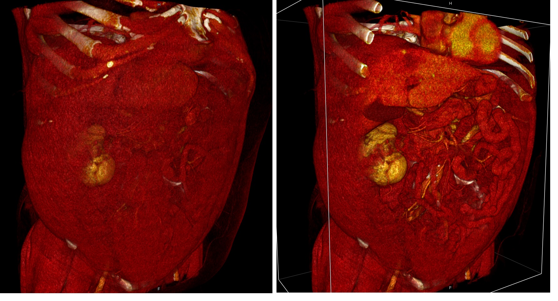
Heart before segmentation and after

Export as a polygonal model opens up another possibility: 3D printing of the exported organ for further analysis, simulation of the operation or even printing of the prosthesis.

In cases where the study is performed for scientific purposes and not for the purpose of medical diagnostics, the segmented model of the organ can be used for various calculations and modeling of the processes occurring in this organ. Although there are techniques in which such calculations are needed already for clinical purposes: for diagnosis and preoperative planning.

How it's done

Basic segmentation tools

One of the most intuitive ways of segmentation of the desired organ is the approach: cut off all unnecessary. To do this, our Inobitec DICOM Viewer has two interactive tools:

Polygon cutting. The tool is applicable only to three-dimensional reconstruction. Two options are possible: delete everything that has fallen into the selected area, or, conversely, delete everything around the selected area.


Using the polygon cut tool

Remove visible tissue with an eraser in the form of a ball or cylinder. The advantage of this tool is its locality: if a polygonal cut always makes a hole “through” and in some cases it is impossible for him to choose such a view so as not to touch the necessary fabrics, then when you remove it with a ball or a cylinder, you can always choose such size , what do you need. In addition, this tool can be used on two-dimensional sections of the MPR-reconstruction, which allows you to immediately get to some hard-to-reach places hidden by surrounding tissues, as well as perform a sheared manual segmentation of the desired organ. This tool has another feature: in the alternative mode, it can restore previously removed tissue from other tools.


Eraser removal

Another intuitive approach is to remove some connected area (for example, a separate bone that is not visually in contact with other bones) or vice versa, except for this connected area. In the Inobitec DICOM Viewer, both of these options are implemented with the appropriate tools (the tools are applicable only to 3D reconstruction). In addition, they have additional options. First, you can set the minimum thickness of the structure that makes the object connected, i.e. if the two parts of the object are connected by some structure whose thickness is less than the specified value, then these two parts will not be considered connected. Secondly, because often, removing voxels by visibility threshold (and visible voxels are classified according to this threshold) leads to a not very natural visualization of editing results, it is necessary to increase one or several voxel layers around the remaining after segmentation - the second parameter allows you to specify the number of such layers. In addition, using the first parameter also cuts off the cusps of objects, which is undesirable in many cases, and increasing the second parameter can help solve this problem.


Deleting Connected Areas

Few technical details needed to understand how other tools work.
Here an important point arises: the appearance of voxels. For a proper understanding of the work of this and other tools, this point requires clarification. How is voxel visualization performed? In the original, all voxels store the density value, but for display, each voxel needs to be assigned some kind of color value and transparency (in our case, this is the RGBA value). The so-called transfer function T is responsible for this:

$$

$$Crgba = T (I),$$

where I is the density value, Crgba is the RGBA value corresponding to this density. Since in reality the stored density values ​​are integer, the function T (I) can be given in tabular form and in this case is called a color table (Color lookup table - CLUT). The transfer function can be arbitrary and each type of transfer function corresponds to a separate color table. Depending on the selected color table, the three-dimensional reconstruction will look different: the densities of one range, corresponding to one type of fabric, can be hidden, and the densities of other ranges, on the contrary, can be made visible and painted in the selected color. Thus, different color tables allow visualization of different organs and tissues, or the same organs in a different way. In addition, color tables can be parameterized depending on the value of the current density window - this is convenient, since it allows you to select the visibility of the desired organs and tissues interactively by changing the width and level of this window.


The same volume visualized using different color tables.

What does all this mean for segmentation? As can be seen in the example of the previous tool, the boundaries of the structure are determined, including on the basis of the current visualization. If two areas of the volume are connected when visualizing using the same color table (for example, the bones are connected by tendons and muscles), then when changing the color table they may not be connected (if only bones are visualized). Thus, the color table and the current density window (since the color table may depend on it, as described above), are the parameters that determine the current segmentation.


Connected and disconnected object depending on the selected color table

Another parameter defining the current segmentation is the visibility mask. What it is? Above, we described the tools that allow you to remove excess tissue. But how does this delete happen? It is performed using a visibility mask. In this mask, each voxel corresponds to one bit, which, respectively, can have the value 0 - the voxel is deleted, 1 - the voxel is not deleted. Thus, tools that remove excess tissue simply set the mask to zero for the voxels to which they are applied. When using a visibility mask, it becomes possible to hide organs and tissues regardless of the color table selected for visualization.

Thus, the current segmentation is determined by three parameters: a color table, a density window, and a visibility mask. If you change any of these parameters, the segmentation may change.
It is probably worth saying here that in this case it is understood by the term “current segmentation” - it means the result of the segmentation process achieved so far. This result is also presented in the form of a bit mask - the same as the visibility mask. Only in this case, a single value of the voxel mask means that it belongs to a segmented object, and a zero value, respectively, has the opposite meaning - the voxel does not belong to the segmented object. It is clear that if the voxel visibility mask has a zero value, then it will always also have a zero value in the segmentation mask. But what value in the segmentation mask will have the voxel, which has a single value in the visibility mask, depends on the color table. This is determined based on the transparency value obtained from the color table for the density corresponding to the voxel: the voxel belongs to the segmentation if the transparency value is greater than a certain threshold. The threshold value can be set in the settings and usually it is 1-10% (100% is completely opaque voxel, 0% is completely transparent). The need to use the threshold is due to the fact that when rendering, voxels with a transparency value less than a certain value are practically invisible, as a result of which a segmentation result may occur that the user sees on the screen.

Segmented structures

Now, when, with the basic concepts of the segmentation process, I hope, more or less clear, the question arises: what to do after we have segmented the organ or pathology we need? Probably, to analyze it, since this no longer interferes with the surrounding tissues and organs. But what if we want to segment several objects and visualize them together? Or what to do in the case when it is easier to segment what hinders viewing, and then hide it? The answer to these and other questions are segmented structures.

A segmented structure is a saved result of segmentation that can be edited and visualized independently. If we need to visualize several organs together, we should sequentially segment each of them and save each as a segmented structure. If we need to remove some object, we should segment it, save it as a segmented structure, and then subtract this segmented structure from the rest of the volume.

How is this implemented? In our Inobitec DICOM Viewer there is a special button that opens a panel with a list of segmented structures. The program has two windows, where there is a panel of segmented structures: a three-dimensional reconstruction window and an MPR viewing window. The logic of working with segmented structures in these windows is somewhat different.


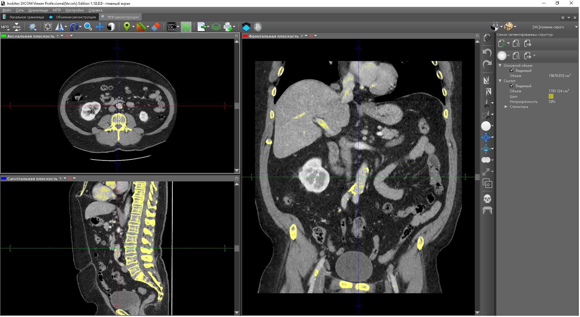
Panel segmented structures on MPR


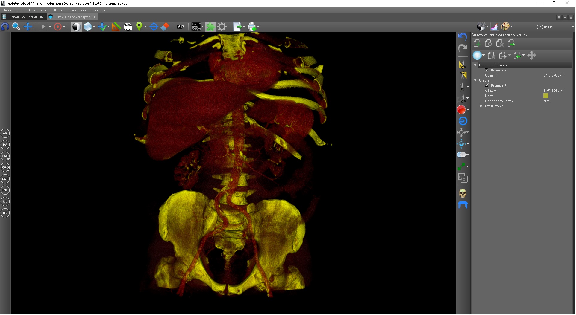
Panel of segmented structures in 3D

In the list of segmented structures there is always a line that cannot be deleted: the base volume. In the three-dimensional reconstruction window, the base volume can be edited to remove excess tissue. The base volume cannot be edited in the MPR viewing window; only the remaining segmented structures can be edited.

Creating a new segmented structure in the 3D reconstruction window occurs by copying the current base volume segmentation option: the current visibility mask, the color table and the density window borders are copied. In the MPR viewing window, a new segmented structure is always created with an empty visibility mask, and the color table and density window are specified in the dialog that appears when creating a new structure. In this dialog, the color table and density window can be specified implicitly - for example, by setting the density threshold value and specifying which voxels will be visible - those that are lower than this threshold or higher. Or specify the boundaries of the density range within which the voxels will be visible. You can also set the color table and the density window value directly. Since the new segmented structure is always empty in the MPR viewing window, the main way of segmentation here is to add new voxels, unlike the three-dimensional reconstruction window, where, on the contrary, segmentation removes extra voxels. Also, when editing segmented structures in the MPR viewing window, the mask of voxels visible when using the current color table and density window is always displayed (not to be confused with the visibility mask described above), for example, if you specify the density threshold and the range of values ​​when creating the structure density above this threshold, the mask will highlight all voxels above this threshold. The transparency of this mask can be customized, including making it completely transparent.


Mask on MPR

Each segmented structure can be hidden or displayed at any time. Also for each segmented structure its volume is shown - thus, by segmentation it is possible to measure the volumes of organs and structures. For all segmented structures, except for the base volume, statistics are calculated: the minimum and maximum density values ​​in the structure, as well as its average value and the standard deviation of this value. Any segmented structure, except for the base volume, can be set to color - in this case, in the color table used, all color values ​​change to the specified (transparency does not change, therefore the segmentation does not change, since it depends only on the transparency, but not on the color ). This is convenient, since often several segmented structures have a common color table and setting a color helps to distinguish them without the need to assign a different color table to each segmented structure.


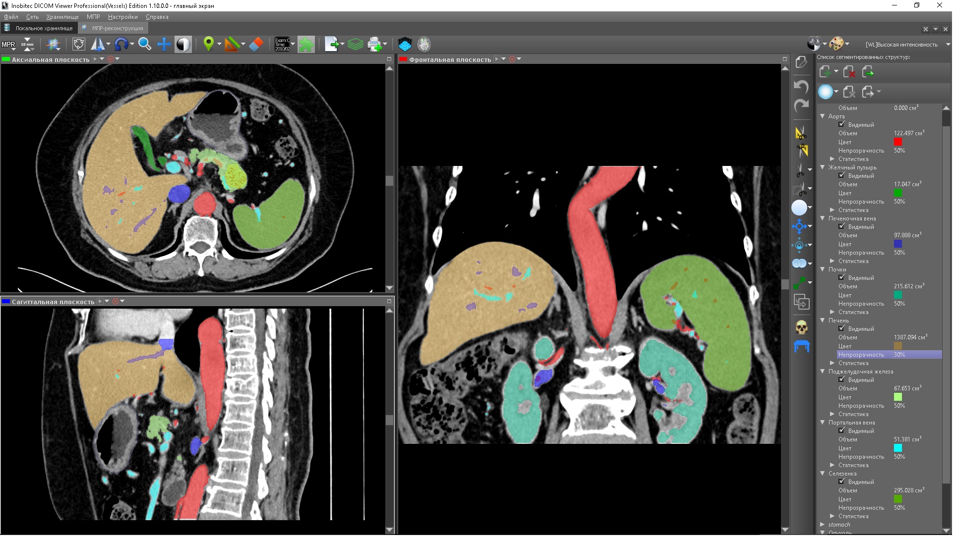
Color segmented structures

Polygonal models

Based on any segmented structure, you can build its polygonal model (grid) - piecewise approximation of the surface of the segmented structure by polygonal elements (triangles). This is one of the important results of segmentation, since almost any software that works with three-dimensional models implies a polygonal mesh as a three-dimensional model. Such software includes visualization, editing, numerical modeling and 3D printing. That is, the export of segmentation results in the form of a polygonal model allows you to work with these results in most third-party programs.

To build grids, the “marching cubes” algorithm is used, which is both simple and most effective for this task. Since the voxel model consists of cubic voxels, when approximating its surface, this “cubicity” is preserved and the grid looks “graded”. To get rid of this, the grid can be smoothed. Smoothing is performed by the Laplace method, which consists in the fact that the coordinates of each vertex of the grid are replaced by the averaged coordinate of all adjacent vertices. The procedure can be repeated several times - each new pass makes the grid more smooth. The number of passes can be set in the grid generation parameters. But it must be remembered that each pass changes the grid, and slightly deviates it from the real surface boundary - the more passes, the greater the deviation. In addition, in some cases, as a result of smoothing, the intersection of grid elements is possible (in fact, the intersection of the surface with itself) or the appearance of triangles with zero area. For some tasks this may be unacceptable, so a large number of smoothing passes must be set with care.


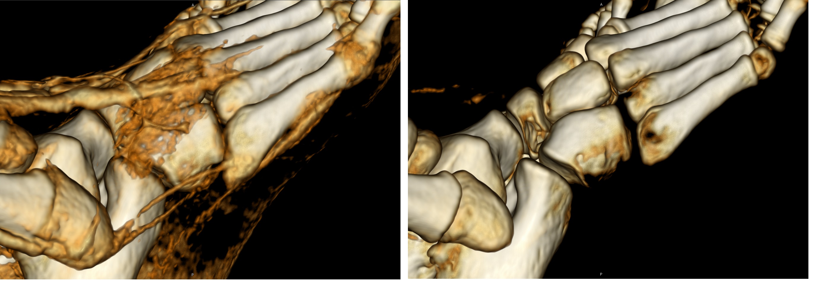
Smoothed and Smoothed Mesh

Also in the parameters for constructing a polygonal surface, you can specify the maximum number of triangles forming the grid. This may be necessary, for example, to speed up the rendering. If this parameter is set (nonzero, zero means that the maximum number of triangles is not limited), then if the number of triangles after the grid has been created by the “marching cubes” algorithm exceeds the specified value, the procedure of sequential combining of triangles will be performed to reduce their total number to required value. But, in some cases, if the required number of triangles is small enough, at a certain point, the merging of the triangles cannot be done without changing the grid topology. In this case, the resulting number of triangles will be equal to the minimum value that can be achieved without changing the grid topology.

Polygonal models can be not only exported, but also imported as segmented structures. In this case, a special type of segmented structure is created - it contains only the imported mesh and no segmentation mask is defined for it. Importing polygonal models can be useful for planning operations — importing models of surgical instruments, accessories, prostheses and implants allows visualizing them together with anatomy and preliminarily evaluating the process or result of the operation. For imported models, a manual positioning tool is available, allowing them to be placed in the desired place and in the desired orientation together with a three-dimensional reconstruction of the anatomy. In addition, segmented structures containing only a mesh can be voxelized. That is, a visibility mask will be created for them, containing only voxels inside the volume bounded by the grid surface. This technique can be used to save and restore the segmentation results: a grid is built for the segmented structure, after which it is exported, and if you open the same study later, the grid can be imported and voxelized, with the result that the segmented structure is restored.

Binary operations on segmented structures

As mentioned above, sometimes there are situations when it is easier first to segment not directly what we need, but instead to segment some secondary objects: for example, something extra that needs to be removed, or separate parts of the whole structure, and then execute over this some additional operations: subtract what you need to remove or merge the parts into a whole. Such operations are called binary. In Inobitek DICOM-Viewer 3 types of binary operations with segmented structures are implemented:

• subtraction
• Union
• intersection

In any of these operations, two segmented structures are involved (one of which may be the base volume). One of these two segmented structures is the target: the result of the operation will be placed in it. The target is always the current active segmented structure. The second structure is optional. When performing operations, the visibility mask of the target structure is modified, but the segmentation masks of the structures, and not their visibility masks, are involved in the operation itself. That is, operations are performed based on current color tables.

When subtracting, all voxels of the segmentation mask of the additional structure are subtracted from the visibility mask of the target structure. That is, it all looks like this, that all visible voxels of the additional structure become invisible in the target structure.


Heart filled with blood, blood filling the heart, myocardium obtained by subtracting

When combined, all voxels of the segmentation mask of the additional structure are added to the visibility mask of the target structure. That is, all the visible voxels of the additional structure are included in the visibility mask of the target structure, but here we must remember that they will not necessarily become visible in the target structure — this already depends on its color table.


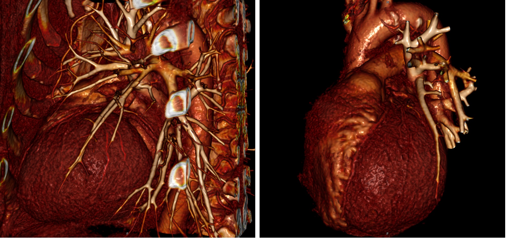
Lung tissue, lung vessels, pool

At the intersection, only voxels are present in the visibility mask of the target structure, which are simultaneously present in the segmentation mask of the target and additional structure. That is, only those voxels of the target structure that are visible at the same time in the target and additional structure remain visible.


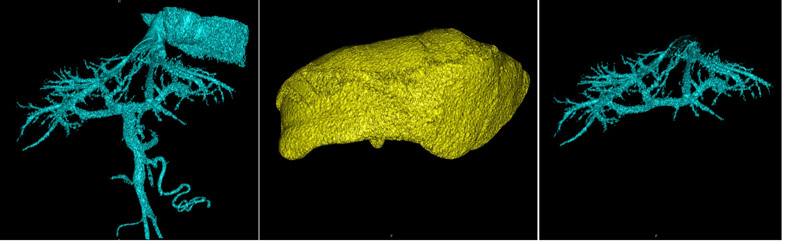
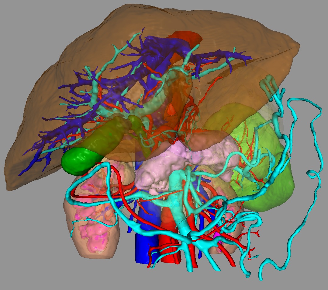
Vessels, liver, their intersection - vessels of the liver

Binary operations are also possible using segmented structures containing only a polygonal model as an extra. In this case, an intermediate voxelization of the polygonal model is performed, with the result of which the binary operation is performed.

Other segmentation tools

Although using the tools described above, you can perform almost any segmentation, in some cases it can be unnecessarily time consuming and take too much time. In the Inobitec DICOM Viewer, additional tools are currently implemented to simplify the segmentation process in many cases.

Morphological operations

Morphological operations are a popular image processing tool. The voxel volume is a generalization of the pixel-by-pixel representation of a two-dimensional image to the third dimension; therefore, many operations applicable to two-dimensional images also apply to the voxel volume. This includes morphological operations. The Inobitek DICOM-Viewer has implemented build-up (growth) and erosion (reduction) operations, allowing to increase or reduce the current segmentation by a specified number of voxels. For the convenience of the user, the size of the accrual / reduction is given in millimeters and not in voxels. Separate closure and opening operations are not implemented, but by definition they can be performed through the sequential application of expansion and contraction operations in the right order. In addition, the operation of filling voids in the current segmentation is implemented. It differs from the closure operation in that it is guaranteed to fill in voids of any size, and not only comparable with the size of the extension / contraction during the closure. In addition, this operation does not affect any other voxels other than voxels belonging to voids.

All morphological operations are applied to the visibility mask, so you need to remember that after they are applied, the changes may not be visible if the voxels that are invisible due to the current color table have changed. In such cases, usually morphological operations should be used in conjunction with a change in the color table / density window.


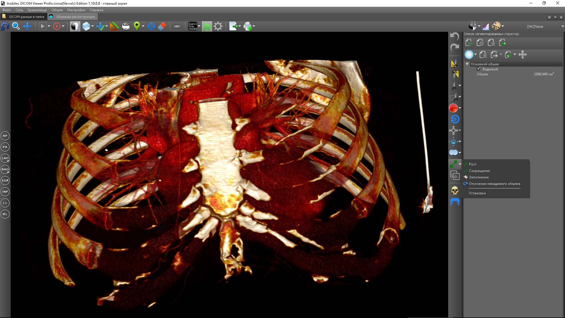
List of morphological operations

In addition to morphological operations, there is one more tool in the list: Removal of invisible volume.

It sets the visibility mask to the current segmentation mask, that is, those voxels that were not hidden by the segmentation mask but were invisible due to the current color table are removed from the visibility mask and become completely invisible, that is, can no longer be made visible by changing color table. The need for such a tool can be illustrated by the following example: suppose we need to segment the bone in a CT scan. Bones have a higher density than other tissues, but the distribution of this density is uneven. The density is higher in the center of the bone and decreases in the direction of its outer border. If by changing the density window or choosing a color table you set a density threshold for visualization equal to the density of the outer border of the bone, then it may not be high enoughespecially in the case of research with contrast - in addition to the bones, some other tissues will be visualized, in particular, contrasted. Therefore, in order to ensure that only voxels belonging to bone structures are visualized, a higher threshold should be established corresponding to the density of the inner bone. But in this case, the bones will be visualized only partially - without external layers. To add external layers, you should apply the expansion operation, but since so far, we have only changed the color table or the density window, our visibility mask corresponds to the entire volume and the capacity will not give anything. Therefore, before building you should remove the invisible volume, then the building will be applied to the visible inner layers of the bone, which will allow you to add to them the outer layers. After that you should change the color table so thatso that the outer layers become visible again - this completes the process of segmentation of the bone structures.

,

The description of interactive segmentation tools has so far largely related to the three-dimensional representation of volume. But as mentioned above, segmentation using MPR slices is also possible. And in many cases it is preferable, as it allows you to quickly get a result.

The main method of segmentation by MPR-slices is: Increasing the volume of the segmented structure within the specified mask. The mask is defined by a color table, and in most cases this color table has the simplest form: it makes visible voxels with a density higher or lower than a given threshold, or within the limits of the specified range. The threshold or boundaries are chosen so as to correspond to the boundaries of the density values ​​of the segmented object. In the process of segmentation, the value of the threshold or boundaries can be interactively changed.


Mask of high density, low density, interval

The basic tool for increasing volume on the MPR is the tool already described above: this is a brush (currently in Inobitek DICOM-Viewer, the brush options are implemented in the form of a sphere and a cylinder of a given size), but when editing in 3D this tool mainly used as an eraser, not a brush. The restoration of the mask with a brush on the MPR theoretically allows you to segment any structure as accurately as possible, but for objects of complex shape it is a very laborious process. The same tool can be used as an eraser not only in 3D, but also on the MPR to remove excess segmented volume. In addition, this tool in brush mode can restore deleted voxels in 3D.


Using the editing tool with a brush.

But in 3D, this tool has another mode - this is mask recovery. The logic of his work is close to that used on the MPR: the tool restores only those voxels that are highlighted with a mask. But since in 3D there is no concept of a mask itself, any other segmented structure must be indicated in its quality (including it is possible to indicate the base volume) that does not coincide with the current segmented structure. To select the structure that serves as a mask, there is a special button on the editing panel.


Using the editing tool with a brush in 3D in the mask recovery mode

Another tool that can be used for segmentation on the MPR is the addition of a coherent area bounded by the mask. To a certain extent, this is analogous to a 3D tool that allows you to segment a connected area, but in this case, instead of deleting everything except the connected area, this connected area is added to the current segmented structure. This tool can also be used in 3D, if a structure is specified, which is a mask. This is a convenient way of segmentation of structures consisting of several unrelated areas — by sequentially applying a tool to each of these areas, all of them can be added to one segmented structure.


Segmentation of isolated areas on the MPR

Region Growth Tool

The above-described tools are opposite to each other in their advantages and disadvantages: using a brush allows segmentation of any object, but often takes a lot of time, adding the same connected area happens with one click, but if the area has even a little contact with any other area or areas, they will be segmented together. Accordingly, a need arises for an instrument devoid of these shortcomings: which could segment areas of arbitrary shape rather quickly.

This tool is a tool for building up the region. The logic of his work is as follows: a certain starting point is selected within the region to be segmented, after that from this point the segmented region is increased according to a certain principle. The build-up takes place under the control of the user and can be stopped at the right moment - when the current segmentation best corresponds to the sementable object. The performance of the tool, expressed in accordance with the required segmentation results, depends on the chosen scaling principle.

The simplest principle is a uniform build-up in all directions within a given mask. But due to this simplicity, this principle has the most pronounced main problem of the tool: leakage. Leakage is called segmentation outside the desired area. For example, if two organs are connected by one or several thin jumpers, during the segmentation of one organ, leakage into another organ occurs through these jumpers, as a result of which it becomes difficult to segment one organ separately from another.


Leaks into surrounding tissues and organs during liver segmentation

Therefore, in reality, the principles of extension with more complex logic are used.
In Inobitek DICOM-Viewer two principles of increasing the region are implemented:
Distance transform ( , , , , ),
(level set).

Distance transform (DT) for a volume is defined as follows: for a binarized volume (binarized, it means that each voxel can have only two values ​​1 - visible or 0 - invisible) in each voxel this transformation gives a value equal to the distance to the nearest visible voxel. The method of measuring the distance can be different, for example, because of the simplicity of the calculations, the so-called Manhattan distance is often used, which is equal to the sum of the distances in each direction. In our case, the classical Euclidean distance is used, so the full transformation is called the Euclidean Distance Transform (EDT). With segmentation using this principle, the volume is binarized on the basis of a mask — in fact, mask inversion is used: voxels falling into the mask have the value 0, the rest 1. Thus,EDT gives the distance to the border of the mask within it. The growth rate is proportional to the EDT value (but only starting from a certain threshold, while the dependence is exponential), as a result, growth in thin structures is slower than in areas with large volume, but it also slows down when approaching the boundaries of the area, which is an undesirable effect. The EDT approach reduces the rate of leakage but cannot completely eliminate it. The main advantage of this approach is high speed operation with acceptable leakage control.but it also slows down as it approaches the boundaries of the area, which is an undesirable effect. The EDT approach reduces the rate of leakage but cannot completely eliminate it. The main advantage of this approach is high speed operation with acceptable leakage control.but it also slows down as it approaches the boundaries of the area, which is an undesirable effect. The EDT approach reduces the rate of leakage but cannot completely eliminate it. The main advantage of this approach is high speed operation with acceptable leakage control.


EDT

. : . — , , , . . : , — , , , , . , , — .

The implementation of this approach is based on the level surfaces method. It is based on the numerical solution of a special type differential equation. The solution of the equation is the function specified at each point of the volume and at the same time dependent on time. The motion of the front boundaries is determined by the surface on which this function takes a zero value. This is a hypersurface in four-dimensional space, but at each moment of time there is its cross section, which is a surface in three-dimensional space - a level surface, hence the name of the method.

The segmentation obtained using the regional extension tool based on level surfaces looks most intuitive. It works well for volume objects, but is not very suitable for segmentation of medium and small vessels - the curvature of their surface is too great.

In this mode, the tool does not use a mask to set the density range; instead, the range is automatically calculated based on the current density window and the initial segmentation point. The tool also allows you to interactively adjust surface curvature parameters that affect the segmentation process. When the tool is turned on, a circle is shown, the radius of which approximately corresponds to the threshold radius of curvature, in other words, the size of this circle approximately corresponds to the minimum size of the structure through which the segmentation can pass. If a leak occurs, the radius of the circle should be increased; if, on the contrary, the structures of the desired size are not segmented, the radius of the circle must be reduced.

The advantage of this tool is its “intelligence” - the results of its work are most intuitive and in many cases it allows you to segment structures of complex shape with minimal labor costs. The disadvantage of the tool is its high computational complexity, but its implementation is quite efficiently accelerated using the GPU, so the use of a powerful video card greatly enhances the interactivity of the tool.


Building the region based on the level surfaces method

Segmentation using multiple tomographic series

Often it is necessary to perform segmentation, which requires data obtained in different tomographic series. A classic example of such a task is the removal of bone structures in a CT series with contrast using a CT series without contrast, obtained immediately before its introduction. The urgency of the task is explained by the fact that the x-ray density of the contrast agent in CT is comparable to the x-ray density of the bone structures, therefore, contrasted vessels that are in direct contact with the bone cannot be separated from it. Since this example is provided for illustrative purposes, we will not consider the problems associated with the movement of the patient between the receipt of these two series. In this case, the task is reduced to the segmentation of the bone structures in the series without contrast and further subtraction of the obtained segmentation from the series with contrast.


, ,

Another example is the joint visualization of arteries and veins with their separate segmentation. In this case, a short time after the introduction of contrast, it spreads through the arteries and at this moment the first series is produced - the arterial phase, in which the arteries are highlighted by contrast. After some time, the contrast is partially washed out of the arteries, passes through the tissues and enters the veins - at this moment the second series is obtained - the venous phase, in which the veins are highlighted by contrast. Thus, using the first series, it is convenient to perform segmentation of the arteries, and using the second series - veins. In addition, if the contrast in the venous series is not completely washed out of the arteries, it can be removed by performing a subtraction of the segmentation of the arteries from the first series. In this way,for joint visualization of veins and arteries, it is necessary to use data from two series - the arterial and venous phases. And if you make another scan before the introduction of contrast, you can perform and remove the bones, in this case, in the joint segmentation will take part already three series.




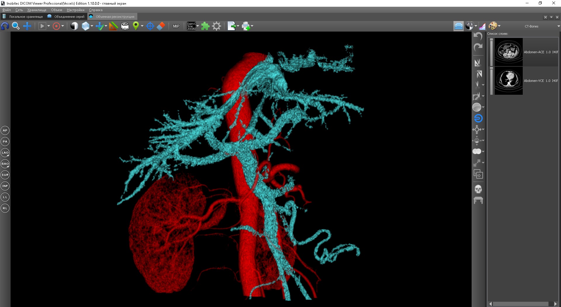
For joint visualization of several series in the Inobitek DICOM-Viewer there is a special mode - series combining mode. You can combine the series in a special window. After combining, an additional virtual series appears in the list of study series, opening which in the required viewing mode (all available viewing modes are supported: 2D, MPR, 3D, virtual endoscopy), you can visualize the selected series together. When viewing such a series, an additional panel appears - the layers panel. Each layer is one of the combined series. The current layer can be changed by selecting the corresponding element on the layers panel. Each series has its own list of segmented structures, so when you change the current layer, the current list of structures also changes.All segmentation operations are applied to the currently selected segmented structure of the currently selected layer. An exception is when the main volume is selected in 3D. In this case, polygon cutting operations and brush operations are applied to all layers at once - this behavior is more intuitive, since when cutting, it is logical to expect that everything in the selected area will be deleted.

Binary operations are possible between segmented structures of different layers. Just with their use, it is possible to subtract bones segmented on one layer from the data of the second layer. If for a user, carrying out a binary operation between structures of different layers on the eye is no different from the same binary operation between structures of one layer, in terms of technical implementation, this is a much more complicated operation. The voxel volumes of different layers may not coincide both in dimension and in their orientation, as well as in the size of the voxel. That is, the voxel of one layer geometrically may not coincide with the voxel of another layer, overlap several voxels at once, or even be outside the model. Therefore, for conducting a binary operation between layers,first, an intermediate interpolation of the segmentation mask of the additional structure onto the target layer is performed, with the result of which the binary operation is performed.

Conclusion

The tools and approaches described in this article are universal and can be used for the segmentation of any objects, organs and formations. With on-line diagnostics or in some other cases, there may be a task of segmentation of the same organs on the basis of data of the same type of research many times in a row. In this case, the use of universal tools may not be the fastest and most convenient way of segmentation and it is easier to use specialized tools in such tasks. A specialized tool can be simply an implementation of a pattern of application of universal approaches, or it can use some algorithms and methods specially developed for a particular case.Currently, we are developing similar tools and plan to continue to talk about their functionality and operating principles as they are implemented.