Dive into pyTorch

Hello. My name is Arthur Kadurin, and I lead research in the field of in-depth training for the development of new drugs at Insilico Medicine . At Insilico, we use state-of-the-art machine learning techniques, and we also develop and publish many articles ourselves in order to cure diseases such as cancer or Alzheimer's disease, and possibly aging as such.

In preparation for my in -depth training course , I am going to publish a series of articles on Adversarial networks with an analysis of what it is and how to use it. This series of articles will not be another review of GANs ( Generative Adversarial Networks ), but will allow you to take a deeper look under the hood of neural networks and cover a wider range of architectures. Although we will also analyze the GANs.

In order to continue discussing the adversarial networks without any further obstacles, I decided to first make a small introduction to pyTorch . I want to immediately note that this is not an introduction to neural networks, so I assume that you already know such words as “layer”, “batch”, “backprop”, etc. In addition to basic knowledge of neural networks, of course, you will need an understanding of the python language.

In order to be comfortable using pyTorch, I prepared a docker container with jupyter and code in laptops. If you want to run training on a video card, then for NVIDIA video cards you need nvidia-docker, I think most of you will have no problems with this part, so I leave the rest to you.

Everything you need for this post is available in my spoilt333 / adversarial repository with the intro tag on the Docker Hub , or in my GitHub repository .

After installing the docker, you can start the container, for example, with the following command:

docker run -id --name intro -p 8765:8765 spoilt333/adversarial:intro 

The jupyter server, which will be available at http://127.0.0.1:8765 with the password "password" (without quotes), will automatically start in the container. If you do not want to run someone else's container on your machine (correctly!), Then you can assemble your own one, after checking that everything is OK there, you can do it from the file that is in the GitHub repository.

If everything started and you were able to connect to jupyter, then let's move on to what pyTorch is. pyTorch is a large framework that allows you to create dynamic computation graphs and automatically calculate gradients from these graphs. For machine learning, this is exactly what you need. But, besides the very possibility of teaching models, pyTorch is also a huge library including datasets, ready-made models, modern layers and communities around it all.

In Deep Learning, for quite a long time, it was practically the standard to test all new models on the task of recognizing handwritten numbers. Dataset MNIST consists of 70,000 handwritten numbers marked up roughly equally distributed between classes. It is immediately divided into training and test sets in order to ensure the same conditions to all who are tested on this dataset. In pyTorch, of course, there are simple interfaces for it. Despite the fact that comparing the state-of-the-art model with each other on this dataset does not make much sense anymore, for demonstration purposes it will suit us perfectly.

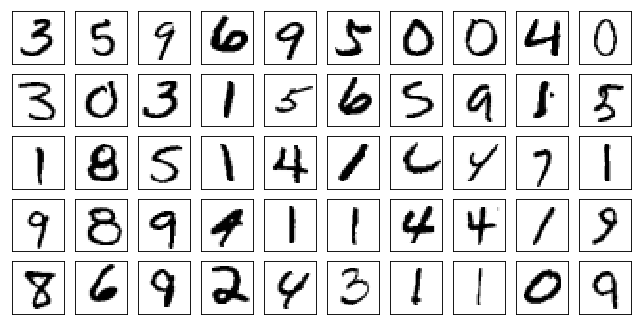
Each example in MNIST is a 28x28 pixel image in shades of gray. And, as it is easy to see, not all figures can easily be recognized even by a person. In the mnist.ipynb laptop, you can look at an example of loading and displaying datasets, and several useful functions are included in the utils.py file. But let's move on to the main "dish".

The mnist-basic.ipynb laptop has a dual-layer fully connected neural network that solves the classification problem. One way to make a neural network using pyTorch is to inherit from the nn.Module class and implement its initialization and forward functions.

 def __init__(self): super(Net, self).__init__() self.fc1 = nn.Linear(784, 100) self.fc2 = nn.Linear(100, 10) 

Inside the __init__ function, we declare the layers of the future neural network. In our case, these are linear layers nn.Linear which have the form W'x + b , where W is the weights matrix of size (input, output) and b is the displacement vector of output size. These very weights will be “trained” in the process of neural network training.

 def forward(self, x): x = x.view(-1, 28*28) x = F.relu(self.fc1(x)) x = self.fc2(x) x = F.softmax(x, dim=1) return x 

The forward method is used directly to convert input data using a given neural network into its outputs. For simplicity of the example, we will work with examples from MNIST not as with images, but as with vectors each dimension of which corresponds to one of the pixels. The view () function is an analogue of numpy.reshape () , it re- indexes the tensor with the given data. " -1 " as the first argument of the function means that the number of elements in the first dimension will be calculated automatically. If the initial tensor x has the dimension (N, 28, 28) , then after

 x = x.view(-1, 28*28) 

its dimension will be equal to (N, 784) .

 x = F.relu(self.fc1(x)) 

Applying layers to data in pyTorch is implemented as simply as possible; you can "call" a layer by passing the data batch as an argument to it and get the result of the conversion. The activation functions are similarly arranged. In this case, I use relu , since this is the most popular activation function in computer vision tasks, however you can easily experiment with other functions implemented in pyTorch, since there are enough of them.

 x = self.fc2(x) x = F.softmax(x, dim=1) 

Since we solve the classification problem into 10 classes, the output of our network has a dimension of 10. We use softmax as the activation function at the output of the network. Now the values ​​returned by the function forward can be interpreted as the probabilities that the input example belongs to the corresponding classes.

 model = Net() optimizer = optim.SGD(model.parameters(), lr=0.01) 

Now we can create an instance of our network and select the optimization function. In order to get a nice training schedule, I chose an ordinary stochastic gradient descent, but in pyTorch, of course, more advanced methods are implemented. You can try for example RMSProp or Adam.

 def train(epoch): for data, target in train_loader: optimizer.zero_grad() output = model(data) loss = F.cross_entropy(output, target) loss.backward() optimizer.step() 

The train function contains the main training cycle in which we iterate over the batches from the training set. data are examples, and target are appropriate labels. At the beginning of each iteration, we reset the current value of the gradients:

 optimizer.zero_grad() 

Data processing by the entire network in pyTorch is no different from the use of a separate layer. The call to the function forward is hidden behind the call to model (data) , so the network outputs fall into the output. Now it only remains to calculate the value of the error function and take a backward propagation step:

 loss = F.cross_entropy(output, target) loss.backward() 

In fact, when calling loss.backward (), the weights of the network are not yet updated, but for all weights used in the error calculation, pyTorch counts the gradients using the constructed graph of calculations. In order to update weights, we call optimizer.step () , which, based on its parameters (we have this learning rate), updates weights.

After 20 epochs of learning, our network guesses numbers with an accuracy of 91%, which, of course, is far from SOTA results, but not bad for 5 minutes of programming. Here is an example from a test set with predicted answers.

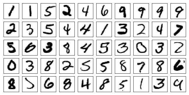
 [[1 1 5 2 4 6 9 9 9 9] [2 3 5 4 4 1 3 2 4 7] [5 0 3 9 4 5 3 2 3 2] [0 3 8 2 5 5 8 7 8 6] [8 3 6 8 4 8 5 1 3 9]] 

In the next posts I will try to talk about adversarial networks in the same style with code examples and prepared docker containers, in particular, I plan to touch on topics such as domain adaptation, style transfer, generative adversarial networks and analyze some of the most important articles in this area.

Upd.1: As correctly indicated in the comments, it is no longer necessary to wrap the tensors in the Variable , so I deleted the corresponding line. It will naturally remain in the docker-container, but everything works without it too.
Upd.2: Pictures with numbers were mixed up in places, so I changed them