We are looking for cycles on the Lorenz attractor in the Maxima package.

This topic continues a series of my articles on Habré devoted to the study of the Lorenz attractor.

Part 1. A critical look at the Lorenz attractor
Part 2. The dynamic Lorentz system and computational experiment
Part 3. On the existence of periodic solutions in the Lorentz system
Part 4. Three cycles in the Lorenz attractor
')
So, consider the nonlinear system of differential equations introduced by Edward Lorenz in 1963:

$$

$$(1) \ left \ {\ begin {array} {l} \ dot {x} = \ sigma (yx), \\ \ dot {y} = rx-y-xz, \\ \ dot {z} = xy-bz, \ end {array} \ right.$$

Where

$$

$$\ sigma = 10, \: r = 28, \: b = 8/3 \: -$$

classical values ​​of system parameters.

For any solution of the Lorentz system, there is a moment in time when the corresponding phase trajectory plunges forever into a sphere of a fixed radius. Therefore, there exists a limit set — the Lorenz attractor — to which all trajectories of a dynamical system attract when time tends to infinity. Thus, the attractor determines the behavior of the solutions of a dynamic system over large periods of time.

In the 70s. Based on the results of numerical experiments, Hookenheimer, Williams and York formulated a hypothesis about the structure of the Lorenz attractor with the classical values ​​of the system parameters; however, this hypothesis was not rigorously proved. In 2000, Steven Smale compiled a list of 18 of the most significant mathematical problems of the 21st century. The problem of the structure of the Lorenz attractor was included in this list under number 14. Warwick Tucker in his 2002 work proved, strictly speaking, the attractor's hyperbolicity in system (1), i.e. the attractor consists of trajectories everywhere dense on it, along which close trajectories run exponentially (continuum of saddle trajectories); this creates their chaotic behavior. Then (as noted by D.V. Anosov in the afterword to the book by G. Palis and V. de Melu "Geometric theory of dynamical systems", Mir, 1986, p. 285) in the attractor of system (1) " may (and not rarely) ) there are an infinite number of asymptotically stable periodic trajectories ", but, in my opinion, their region of attraction can be quite small (difficult to capture in a numerical experiment). Based on the calculations in the work of VS Afraimovich, V.V. Bykova and L.P. Shilnikov, “On the Origin and Structure of the Lorenz Attractor” (DAN SSSR, 1977. –T. 234, No. 2, p. 336-339), the structure of the attractor is described - it contains an everywhere dense set of saddle cycles.

How do you usually track loops in the Lorenz system? They use symbolic dynamics — they divide a region in the phase space containing an attractor into a finite number of subdomains. Denoting each element of the partition of the letter, the trajectories on the attractor, passing through the corresponding areas, are encoded by sequences of such characters. If there is a regularity in the sequence — the recurrence of groups of characters — then we are dealing with a cycle. However, the return of the trajectory to a certain neighborhood of its part does not indicate its closure (part 1). In general, a criticism of the results of such computational experiments can be found in the scientific literature (see, for example, Chapter 4, “ Rene Losey, written by the French mathematician and published in 2013 in the book “ Topology and Dynamics of Chaos ” ).

In 2004, Divakar Vishwanath published “The fractal property of the Lorenz attractor” (Physica D: Nonlinear Phenomena, 2004. - Vol. 190, iss. 1-2, pp. 115-128), in which he cited initial conditions and periods for three cycles in the Lorenz attractor. In my opinion, this work became revolutionary in chaotic dynamics, because the author for the first time showed specific values ​​of phase coordinates and period with a sufficiently high accuracy. The calculation algorithm was based on the method of Lindstedt-Poincaré (LP), which (unlike the methods of numerical integration) is not affected by the stability of the cycle, to which approximations are constructed.

Particularly impressive is the third cycle.

It may seem that there are several cycles, but no - this cycle has such a multi-spiral structure due to the dominance of a large number (about 100) of harmonics.

Analysis of the work of Viswanath showed that the author provides a description of the algorithm without software implementation (in MATLAB, as written in his articles). At the same time, it is not clear how the resulting inhomogeneous linear system of differential equations with periodic coefficients is symbolically solved for the LP method (for example, for the van der Pol equation this can be done without special problems). The author does not respond to the letters with the request to send the source texts of the programs. It can be understood - he cited data that can be checked (part 4), solving the Cauchy problem with highly accurate numerical methods (part 2), and how exactly everything is done - the algorithm is already closed, reserving the right of sole authorship. A search for works on citations showed that later no one reproduced the Vishwanath algorithm for finding periodic solutions in the Lorentz system.

Therefore, the idea of ​​an open project emerged, where everyone can download the source code of the program and find new cycles in the Lorentz system. In this topic, I will describe the algorithm of the programs, which, by the way, requires further improvement in speed, but one cycle has already been received. It is interesting to find order among the chaos. ;)

Fourier Series Method

Since there are still ambiguities with the LP method, it was decided to try the Fourier series method for the nonlinear system (1) with the sliper01 feed. To do this, we make an approximation of the phase coordinates on the period by trigonometric polynomials in general form with an unknown cyclic frequency (since we do not know the value of the period of the desired periodic solution; in general, it may be an irrational number):

$$

$$\ begin {array} {l} \ displaystyle x (t) \ approx \ tilde {x} _1 (t) = x_ {10} + \ sum_ {i = 1} ^ h c_ {1, i} \ cos ( i \ omega t) + s_ {1, i} \ sin (i \ omega t), \\ \ displaystyle y (t) \ approx \ tilde {x} _2 (t) = x_ {20} + \ sum_ {i = 1} ^ h c_ {2, i} \ cos (i \ omega t) + s_ {2, i} \ sin (i \ omega t), \\ \ displaystyle z (t) \ approx \ tilde {x} _3 (t) = x_ {30} + \ sum_ {i = 1} ^ h c_ {3, i} \ cos (i \ omega t) + s_ {3, i} \ sin (i \ omega t), \ end {array}$$

where h is the specified number of harmonics.

By virtue of the right side of system (1) we make up the residuals

$$

$$\ begin {array} {l} \ delta_1 (t) = \ tilde {x} '_ 1 (t) - \ sigma [\ tilde {x} _2 (t) - \ tilde {x} _1 (t)], \\ \ delta_2 (t) = \ tilde {x} '_ 2 (t) - [r \ tilde {x} _1 (t) - \ tilde {x} _2 (t) - \ tilde {x} _1 (t) \ tilde {x} _3 (t)], \\ \ delta_3 (t) = \ tilde {x} '_ 3 (t) - [\ tilde {x} _1 (t) \ tilde {x} _2 (t) - b \ tilde {x} _3 (t)], \ end {array}$$

where the derivative of the function with respect to time is redefined. If you perform calculations in analytical form on paper for a small number of harmonics (2-3), then for each residual you need the following:

1. Differentiate in time the corresponding trigonometric polynomial;
2. Where there are products of phase coordinates, multiply them by transforming the products of trigonometric functions into sums;
3. Give similar terms for each function cos () and sin () with the corresponding argument;
4. Since we are working with the number of harmonics equal to h , we cut off the higher order harmonics from the resulting residual;
5. Equate the resulting discrepancy to zero, i.e. coefficients at its harmonics.

If we put together the algebraic equations found for each residual, we obtain the non-closed system of nonlinear equations for unknown amplitudes, constant terms, and cyclic frequency. The number of unknowns in the system is

$$

$$3 (1 + 2h) + 1 = 6h + 4,$$

and equations - one less.

An additional equation can be taken from the following considerations. In the above literature (and not only) track the intersection of the trajectories on the attractor with the plane (or subdomains through which it passes), where the equilibrium positions of the system

$$

$$O_1 \ left (- \ sqrt {b (r-1)}, \, - \ sqrt {b (r-1)}, \, r-1 \ right), \: \: O_2 \ left (\ sqrt {b (r-1)}, \, \ sqrt {b (r-1)}, \, r-1 \ right),$$

parallel to the xOy plane (Poincare section). Thus, the third coordinate in the initial condition for the desired cycles is equal to the value of r -1, whence

$$

$$\ tilde {x} _3 (0) = r-1,$$

then the additional equation of the system has the form:

$$

$$x_ {30} + \ sum_ {i = 1} ^ h c_ {3, i} -27 = 0.$$

I have not met any other additional information about periodic solutions in the Lorentz system. I note that for the three cycles found by Vishwanath, in the initial condition of the third coordinate, the number 27 was taken.

The following is an example of a system of equations for h = 2:

$$

$$\ left \ {\ begin {array} {l} \ omega s_ {1,1} -10c_ {2,1} + 10c_ {1,1} = 0, \\ -10s_ {2,1} + 10s_ { 1,1} -c_ {1,1} \ omega = 0, \\ 2 \ omega s_ {1,2} -10c_ {2,2} + 10c_ {1,2} = 0, \\ -10s_ {2 , 2} + 10s_ {1,2} -2c_ {1,2} \ omega = 0, \\ 10x_ {10} -10x_ {20} = 0, \\ c_ {1,1} x_ {30} + c_ {3,1} x_ {10} + \ dfrac {s_ {1,1} s_ {3,2}} {2} + \ dfrac {s_ {1,2} s_ {3,1}} {2} + \ omega s_ {2,1} + \ dfrac {c_ {1,1} c_ {3,2}} {2} + \ dfrac {c_ {1,2} c_ {3,1}} {2} + c_ {2.1} -28c_ {1,1} = 0, \\ s_ {1,1} x_ {30} + s_ {3,1} x_ {10} + \ dfrac {c_ {1,1} s_ { 3.2}} {2} - \ dfrac {c_ {1,2} s_ {3.1}} {2} + s_ {2,1} + \ dfrac {c_ {3.1} s_ {1,2 }} {2} - \ dfrac {c_ {3,2} s_ {1,1}} {2} -28s_ {1,1} -c_ {2,1} \ omega = 0, \\ c_ {1, 2} x_ {30} + c_ {3,2} x_ {10} - \ dfrac {s_ {1,1} s_ {3,1}} {2} +2 \ omega s_ {2,2} + \ dfrac {c_ {1,1} c_ {3,1}} {2} + c_ {2,2} -28c_ {1,2} = 0, \\ s_ {1,2} x_ {30} + s_ {3 , 2} x_ {10} + \ dfrac {c_ {1,1} s_ {3,1}} {2} + s_ {2,2} -28s_ {1,2} + \ dfrac {c_ {3,1 } s_ {1,1}} {2} -2c_ {2,2} \ omega = 0, \\ x_ {10} x_ {30} + x_ {20} -28x_ {10} + \ dfrac {s_ {1 , 2} s_ {3,2}} {2} + \ dfrac {s_ {1,1} s_ {3,1}} {2} + \ dfrac {c_ {1,2} c_ {3,2}} {2} + \ dfrac {c_ {1,1} c_ {3,1}} {2} = 0, \\ -c_ {1,1} x_ {20} -c_ {2,1} x_ {10} + \ omega s_ {3,1} - \ dfrac {s_ {1,1} s_ {2,2}} {2} - \ dfr ac {s_ {1,2} s_ {2,1}} {2} + \ dfrac {8c_ {3,1}} {3} - \ dfrac {c_ {1,1} c_ {2,2}} { 2} - \ dfrac {c_ {1,2} c_ {2,1}} {2} = 0, \\ -s_ {1,1} x_ {20} -s_ {2,1} x_ {10} + \ dfrac {8s_ {3,1}} {3} - \ dfrac {c_ {1,1} s_ {2,2}} {2} + \ dfrac {c_ {1,2} s_ {2,1}} {2} - \ dfrac {c_ {2,1} s_ {1,2}} {2} + \ dfrac {c_ {2,2} s_ {1,1}} {2} -c_ {3,1} \ omega = 0, \\ -c_ {1,2} x_ {20} -c_ {2,2} x_ {10} +2 \ omega s_ {3,2} + \ dfrac {s_ {1,1} s_ {2,1}} {2} + \ dfrac {8c_ {3,2}} {3} - \ dfrac {c_ {1,1} c_ {2,1}} {2} = 0, \\ -s_ {1,2} x_ {20} -s_ {2,2} x_ {10} + \ dfrac {8s_ {3,2}} {3} - \ dfrac {c_ {1,1} s_ {2,1} } {2} - \ dfrac {c_ {2,1} s_ {1,1}} {2} -2c_ {3,2} \ omega = 0, \\ \ dfrac {8x_ {30}} {3} - x_ {10} x_ {20} - \ dfrac {s_ {1,2} s_ {2,2}} {2} - \ dfrac {s_ {1,1} s_ {2,1}} {2} - \ dfrac {c_ {1,2} c_ {2,2}} {2} - \ dfrac {c_ {1,1} c_ {2,1}} {2} = 0, \\ x_ {30} + c_ { 3.1} + c_ {3,2} -27 = 0. \ end {array} \ right.$$

A cursory analysis for three or more harmonics showed that finding the general formulas for some of the equations of the system is still difficult. Note that for any h such a system has solutions

$$

$$\ begin {array} {c} \ displaystyle x_ {10} = x_ {20} = \ pm \ sqrt {b (r-1)}, \: x_ {30} = r-1, \: c_ {k , i} = 0, \: s_ {k, i} = 0, \\ \ omega \: - \: \ mbox {any number}, \: \, k = \ overline {1,3}, \: i = \ overline {1, h}, \ end {array}$$

corresponding to the specified equilibrium positions.

Maxima Symbolic Computation Package

So, to get an approximation to a periodic solution, we must obtain a nonlinear system with respect to the unknown expansion coefficients and frequencies. As can be seen from the above example, even for two harmonics, the system has a cumbersome look. Therefore, we consider an algorithm for performing symbolic calculations to obtain it.

When developing the project, I chose the Maxima math package. The input_maxima.wxm file with the amplitude and constant term residual instructions for h = 2 is presented below.

/* [wxMaxima batch file version 1] [ DO NOT EDIT BY HAND! ]*/
/* [wxMaxima: input start ] */
display2d:false$
x1:x10+c1c1*cos(1*omega*t)+s1c1*sin(1*omega*t)+
c1c2*cos(2*omega*t)+s1c2*sin(2*omega*t)$
x2:x20+c2c1*cos(1*omega*t)+s2c1*sin(1*omega*t)+
c2c2*cos(2*omega*t)+s2c2*sin(2*omega*t)$
x3:x30+c3c1*cos(1*omega*t)+s3c1*sin(1*omega*t)+
c3c2*cos(2*omega*t)+s3c2*sin(2*omega*t)$
assume(omega > 0)$
delta1:trigreduce(diff(x1,t)-(10*(x2-x1)),t)$
delta2:trigreduce(diff(x2,t)-(28*x1-x2-x1*x3),t)$
delta3:trigreduce(diff(x3,t)-(x1*x2-8/3*x3),t)$
expand(diff(delta1,cos(1*omega*t)));
expand(diff(delta1,sin(1*omega*t)));
expand(diff(delta1,cos(2*omega*t)));
expand(diff(delta1,sin(2*omega*t)));
expand(integrate(delta1,t,0,2*%pi/omega)*omega/(2*%pi));
expand(diff(delta2,cos(1*omega*t)));
expand(diff(delta2,sin(1*omega*t)));
expand(diff(delta2,cos(2*omega*t)));
expand(diff(delta2,sin(2*omega*t)));
expand(integrate(delta2,t,0,2*%pi/omega)*omega/(2*%pi));
expand(diff(delta3,cos(1*omega*t)));
expand(diff(delta3,sin(1*omega*t)));
expand(diff(delta3,cos(2*omega*t)));
expand(diff(delta3,sin(2*omega*t)));
expand(integrate(delta3,t,0,2*%pi/omega)*omega/(2*%pi));
/* [wxMaxima: input end ] */

Consider it in more detail. Comments at the beginning and end are needed so that the file can be opened in the latest wxMaxima graphic frontend. The display2d: false $ expression turns off multi-line drawing of fractions, powers, etc. The $ sign allows you to calculate the result of an expression, but not display it (instead of ; ). The trigreduce function (expression, t) collapses all products of trigonometric functions with respect to the variable t in a combination of sums. Differentiation of residuals by harmonic functions is necessary to obtain the corresponding amplitudes. The expand function (expression) opens parentheses (performs multiplication, exponentiation, results in similar terms). To find the permanent terms of the residuals, the integration is applied on the period the constant term of the k -th residual is

$$

$$\ dfrac {\ displaystyle \ omega \ int_ {0} ^ {\ frac {2 \ pi} {\ omega}} \ delta_k (t) dt} {2 \ pi}.$$

In order for a symbolic integration package not to ask a question about the sign of the frequency, the command is given

assume(omega > 0)$

Similarly, the file input_maxima.wxm is formed for any number of harmonics. After executing this script, the package will display in the console symbolic expressions for the left side of the system of algebraic equations, which I solved in it by the Newton method . For example, for five harmonics, the script file newton.wxm is as follows:


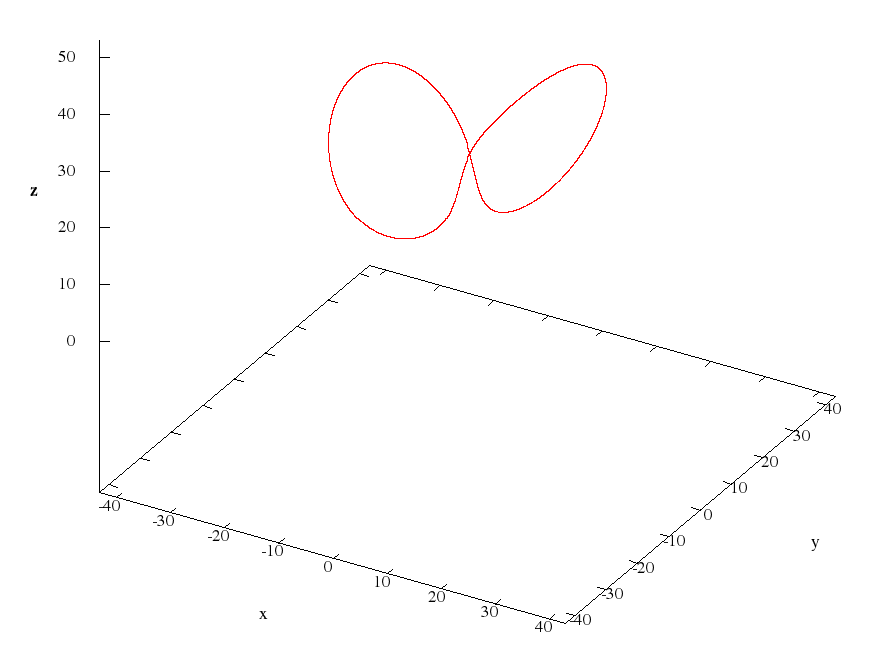
This script is given due to the fact that among the numerous selections of initial approximations for Newton's method, one was found which gives an approximation to the first Vishwanath cycle (the first figure in this topic, part 4). The result of the script are the following values:

(%o3) [[omega = 3.984915779315225,x10 = -1.0530814406427574E-19,
x20 = -1.0530848010639959E-19,x30 = 23.17484126777741,
c1c1 = -5.73442859974501,s1c1 = 8.700967706873968,
c1c2 = -6.138073055934428E-19,s1c2 = -7.0677320406008846E-19,
c1c3 = 3.162874335852723,s1c3 = 2.061936729442591,
c1c4 = -8.5085912287645265E-19,s1c4 = 4.9192865298350146E-19,
c1c5 = 0.52386925730497,s1c5 = -0.691987635106,
c2c1 = -2.267166248701582,s2c1 = 10.98608920812201,
c2c2 = -1.210031439700999E-18,s2c2 = -2.9446761267244605E-19,
c2c3 = 5.627867598584345,s2c3 = -1.719199625236613,
c2c4 = -1.5456862362288386E-19,s2c4 = 1.8698116859813374E-18,
c2c5 = -0.8548869658075,s2c5 = -1.735775069972357,
c3c1 = -3.7683970563654851E-19,s3c1 = 5.9125298542126567E-19,
c3c2 = 7.278395231560698,s3c2 = -9.743072005078496,
c3c3 = 1.1948226901634459E-18,s3c3 = 1.5220232872406872E-18,
c3c4 = -3.45323649933811,s3c4 = -1.496599920543623,
c3c5 = 9.6317779065317723E-19,s3c5 = -1.0610022378452297E-18]]

The period corresponding to the calculated frequency is 1.576742309033. Received initial condition

x(0) = -2.047685006587,
y(0) = 2.505814384075,
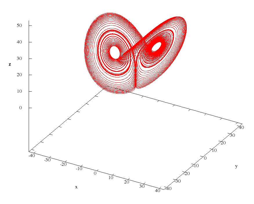
z(0) = 27.

For 20 harmonics, the results are as follows:


Here, the accuracy of the representation of a real number is 30 significant digits after the dot, the command of the packet

(fpprec:30,newtonepsilon:bfloat(10^(-fpprec+5)))$

Then the obtained period T = 1.558652211165 (8 characters after the point coincided with the value indicated by Vishwanath), the initial condition

x(0) = -2.147375914135,
y(0) = 2.078143036771,
z(0) = 27.

The verification of these numbers should be done by numerical solution of the Cauchy problem (for large periods of time go to high-precision calculations). I use the power series method to construct unstable solutions of the Lorentz system, described in part 2. Accuracy of the series took 1E-14, 80 bits under the mantissa of a real number. I will give the values ​​of phase coordinates calculated through the period:

x(T) = -2.147466991199,
y(T) = 2.078421751536,
z(T) = 27.000633876853.

Increasing the accuracy of the series does not have a significant effect on the values ​​obtained. As can be seen, due to the instability of the desired solution (especially at large intervals of time), a sufficiently large number of harmonics must be taken.

In Newton's method, the main problem is the choice of the initial approximation, and for our problem, when it is selected, the method frequently converges to solutions corresponding to equilibrium positions. If a negative frequency value is obtained, then this is a symmetric solution — by changing its sign, we change the signs to opposite ones for the sine coefficients.

Automation of calculations

Since we are dealing with a cumbersome system of equations, we need programs that will generate scripts for Maxima, run the package and read the results of the calculations. Such programs were written in C ++. All source codes, and also scripts for a packet, are collected in the periodic_sols project on GitHub . We analyze them.

The interaction with the package will be through the redirection of input / output to files. An example of the command to start the package:

 maxima < input_maxima.wxm > output_maxima.txt 

To read commands from a text file, there is a ReadFromMaxima () function (files maxima.h and maxima.cpp ).

 void ReadFromMaxima(std::fstream &f, std::string &res) { std::string s; res = ""; while(1) { f >> s; if(s[1] == '%' && s[2] == 'o') { while(1) { f >> s; if(s[1] == '%' && s[2] == 'i') break; res += s; } break; } } } 

The first argument is a stream associated, for example, with the file output_maxima.txt , the second is a string into which the result is counted. If it is multi-line (Maxima breaks long lines into parts), then the resulting lines are glued together in one line. To run the package, use the standard library function system () from cstdlib .

The periodic_sols project consists of three programs: periodic_sols.cpp , init_newton.cpp, and calc_init_point.cpp . To build them run

 ./compile 

Before running ./periodic_sols, you need to prepare the files input.txt and system.txt . The format of the first file (I did not bother with the interface - all programs are console):

The first line is the order of the system (in our case it is equal to 3, it is stored in the program in the variable n , this is done not only for the system in question);
2nd line - the number of harmonics;
3rd line - the accuracy of the representation of a real number;
4th line - the number of the phase coordinate for the additional equation (in our case it is equal to 3);
The 5th line is the value of this coordinate (in our case it is 27);
The 6th line is the initial approximation in frequency;
The 7th row is the initial approximation for the permanent members;
The 8th line is the initial approximation in terms of cosine amplitudes (0 is taken in sine).

The system.txt file contains the right part of the dynamic system:

10*(x2-x1)
28*x1-x2-x1*x3
x1*x2-8/3*x3

The result is the file newton.wxm with commands for the Newton method. This file is input to the package. The program init_newton.cpp creates a file new_newton.wxm based on the file newton.wxm , recording there the results of calculations for the previous number of harmonics (the prev_harmonics variable) less than or equal to the current number (the harmonics variable). This is necessary when we want to improve our approach to a periodic solution. Here is the algorithm:

1. Having solved a system of nonlinear equations for a small number of harmonics ( prev_harmonics ), we form the file res_newton.txt according to the results of calculations;
2. In the file input.txt, we increase the number of harmonics and run ./periodic_sols to form a new system;
3. Run the program ./init_newton , which transfers the calculated values ​​to the appropriate places of the initial approximation for the new system, and the missing ones are filled with zeros.

The calc_init_point.cpp program, based on the res_newton.txt file , calculates the initial conditions and period by writing to the init_point.txt file. The letter “b” means the same as the letter “E” in the representation of a real number.

What's next?

1. The most time-consuming operation is symbolic integration. For example, for 120 harmonics, the system formation time is more than 2 days. Here you can parallelize the computational process into three nodes, but this will not have a significant effect (Viswanath, in general, calculated 1024 harmonics). Here we need to change the principle of the formation of permanent members. For example, subtract from the general expression obtained before this expression for each harmonic. By the way, when solving a system of nonlinear equations by the Newton method, the Jacobi matrix is ​​not addressed; the package uses the LU decomposition to solve a system of linear equations at each iteration of the method;
2. Now I am looking for analogies in the resulting systems of nonlinear equations for different numbers of harmonics, so that the system is formed immediately. If someone wants to try too, there is an archive with systems for 2-7 harmonics. If you need more, write in the comments, add;
3. The T__undefined directory contains approximations to the as-yet-unknown periodic solution of the Lorentz system (the number directories inside correspond to the number of harmonics found). Not yet counted. If the method for this case nevertheless converges, then the cycle period will be greater than the period of the third Vishwanath cycle;
4. As I wrote above, the main problem of the Newton method is the choice of the initial approximation. If a general view of the system is obtained, it would be good to separate the solutions corresponding to the equilibrium positions from it, i.e. get a new system, the solutions of which are only the desired periodic solutions. Then the initial approximation is much easier to select. Note that the end of the source file, periodic_sols.cpp, contains a comment with initially selected initial approximations for the first cycle of Vishwanath (as it turned out later) and an unknown periodic solution.