Effective online quality assessment in the development of web services. Yandex lecture
The development of services is now based on an assessment of their quality. To assess the user interaction with the product, online experiments are conducted, and only then decisions about launches and updates are made. For example, in 2015, Google conducted up to 1,000 such experiments daily. The number of small companies that use AB testing is growing. At the regular Yandex meeting from the inside, research developer Alexey Drutsa examined the modern mathematical methods underlying the online assessment platforms.
- My report will be about online quality assessment for the effective development of web services. First, I will tell about our team, about what we do.

We in the department of scientific research are engaged in various fields of computer science. This includes data analysis, theoretical foundations of machine learning, processing of natural texts, computer vision and information retrieval, and sometimes it is possible to work on auctions and game theory.

')
Our small department is constantly published at leading conferences in these areas, such as NIPS, ICML, KDD, CVPR, ACL, etc.
Here, only those articles that have been published over the past few years.


In today's report I will talk about one of the areas in which we have been very concentrated in recent years. This is an online assessment of the quality of web services.
Over the past five years, I and my colleagues have been able to make a significant contribution to the development of this subject, we have published 14 articles at leading conferences. One of them received the award for the best article at the leading information search conference in 2015.
Online quality assessment in the development of a web service or product plays a key role in deciding whether to launch new functionality. Let's take a look at how this process works in Yandex.

Dozens of experiments are conducted at any time. An example of the experiment is shown on this slide. We see two options for issuing on the same search query. Next to the results of the issuance of the right there are miniature pictures.
Do you think the right-hand option is better than the left, and improves service? The correct answer will say later.

The slide again shows two options for issuing the same search query. On the right variant there is no factoid.
Do you think the right service option is better than the left one? The correct answer will say later.
The answer to my inquiries strongly depends on what we put into the concept of “improve”. So let's see what is under the hood of AB-testing.
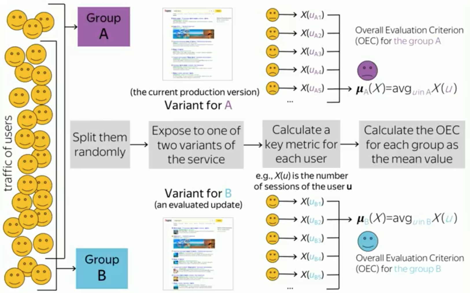
It is useful to recall the key points of support for this process. For each experiment, a certain set of users is allocated that will participate in this experiment. Further, this set is divided randomly into two groups. For example, equally. We define half of the users in group A, and half in group B.
Each of these groups then displays its own version of your website, web service, or product. For example, group A shows the current working version of the product, which is shown to most users, and group B shows the new experimental version of the product, which contains, for example, the new functionality that you want to test.
After the expiration of a certain time, you complete the experiment, for example, in a week or two, and collect some statistics and information about their behavior from all users. For example, it can be one number for each user. This number — for example, the number of user sessions on a site during an experiment — we call the key metric. We aggregate these numbers among all users in each group, and get a number for each of the groups. This is sometimes called an aggregated metric or evaluation criterion. Thus, we get one number for each group. For our example, this is the average number of sessions per user in each group.
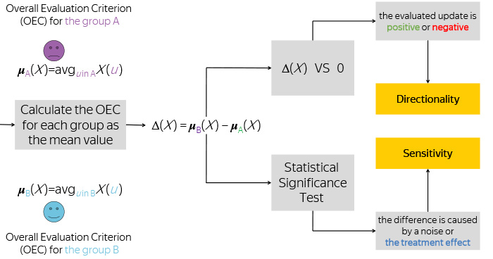
Having these two numbers, we take their difference, and compare this difference with zero, in order to understand whether your metric has changed in a positive or negative direction, and also remember how big this difference was.
But this is not enough for you to know. We all know that the division of users into groups is random, the behavior of users is also completely subject to a random process, and therefore the observation of your difference is a certain random variable. Or the implementation of a random variable.
To understand whether the observed difference differs from the possible noise in the data, we apply a statistical test. For example, it may be the well-known Student's t-test.
After that, we decide whether or not the change we are seeing is a consequence of the new functionality we are testing. Or, this observation is just a noise in the data, but in reality your new functionality has no effect on users, at least in terms of this metric.
These two processes lead us to two key properties or metric definitions that a metric should possess. Let's take a closer look at these two properties.
In reality, the observed difference in the average values of the metric X for versions A and B is an unbiased estimate of the average effect of influence, which in turn is also the difference, but already the expected value of the metric X for version A and version B.
Thus, it must always be remembered that the observed delta is a realization of a random variable. Let's imagine that as a result of the experiment we got a delta equal to one percent increase in the number of sessions per user. Is it a lot or a little? This is indicated on the screen as a large segment. This is probably a very large value.

But in order to understand this, you need to find out if we can observe such a delta if the service versions are indistinguishable. The average effect of the effect is zero.
Often this condition is also called the null hypothesis. Here, everything strongly depends on what the distribution of this is. The screen shows two possible distributions. And it is easy to see that if we are dealing with the distribution of blue, then the probability of observing this delta is much less with the null hypothesis than if we are dealing with the distribution of green.
To understand or be sure of the significance of that observation or the observed change, we calculate the probability of observing this delta or more under the condition of the null hypothesis.
To calculate this probability, as a rule, we use the well-known Student's T-test, which is based on T-statistics.

Here is its formula, in the numerator is the delta, and in the denominator there are two more values. The first value is the variance of the metric X for each of the groups. The second is the sample size of each group. The higher the T-statistics module, the more we are confident of the observed change in our delta.

Let's take a closer look at the conditions under which the T-statistics module will be larger. Consider the expression for T-statistics. It depends on three quantities. It is clear that this module of T-statistics will be higher if the numerator is larger, if the experiment greatly changes the metric. Only under this condition will the numerator be larger. For example, if the experiment will shift the metric by 10%, by 20%, by 30%. What other big numbers can we imagine?
But this happens very rarely when your service has been developing and improving for many years. In addition, the size of the change in the experiment depends on the experiment itself, on the functionality that you are testing. If you are testing functionality that has very little impact on users, then the delta will be very small. Therefore, the numerator is not subservient to us. And therefore, if we want to increase T-statistics, then only the denominator depends on us, only we can change it.
The easiest way is to increase the number of users that we use in the experiment. But this method is bad because it reduces the throughput of the experimental platform, which means its efficiency.
An alternative way is to reduce the variance of the metric. Thus, we gradually come to such a concept as the sensitivity of the metric. For simplicity, we assume that this is the average T-statistics module for all experiments. The higher the sensitivity, the weaker changes we can notice in our experiment. Or alternatively, we can use fewer users in the experiment to observe the same changes that we observed before, but at the same level of significance as with the initial number of users.

The main key to increasing sensitivity is reducing the variance of the metric, which I mentioned earlier.

We turn to the second concept - directional metrics.
Consider two metrics: the number of clicks per user during the experiment and the number of sessions per user. It turns out that in this example, the number of clicks per user increased, which indicates a positive effect. Visitors use output better.
In addition, the number of sessions per user has also increased. This means that users began to return to our site more often to solve everyday tasks.

In the second example, we also observe an increase in the number of clicks, since in the right-hand version of the results there is no factoid on the query that the user asked. Therefore, they should search for this answer, going to the site, and make more clicks. Despite this, the right version of the service without a factor leads to a decrease in the number of sessions per user. And in this example, we see that the click metric of user activity conflicts with a more long-term metric that measures user loyalty, and therefore more suitable for an urgent purpose.
In the end, what do we have? The number of clicks is increased, and the number of sessions is reduced in the experiment.
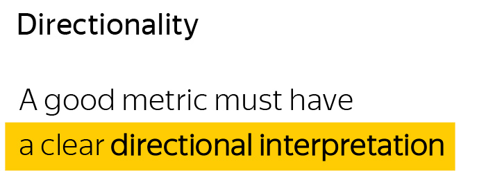
To sum up briefly, we call a good metric one that has a clear interpretation of the directions of its change or direction. And this is a key criterion when choosing a metric. Without this property, it is very difficult for any analyst to make the right conclusion, to make the right decision about the success or failure of the test update or functionality.
Consider some class of user enthusiasm metrics for example. As a rule, two groups of metrics are assigned to this class of metrics. The first group is loyalty metrics, such as the number of sessions per user, the time of his absence, etc. The second group consists of activity metrics. These are such metrics as the number of user clicks, the number of user requests, the time spent on the site, etc.
The first category of metrics has a very good focus. The interpretation of its changes is very transparent and, as a rule, correlates with the company's long-term goals for long-term existence and development.

At the same time, these metrics have very low sensitivity. In our experiments, such metrics are very difficult to move, it is very difficult to invent a new functionality that will significantly increase user loyalty or the number of tasks that they solve in their daily life through our service.
On the contrary, activity metrics have a confused direction, but at the same time they have a very high sensitivity. They are very easy to move. Any experiment that introduces functionality that changes or affects the design, immediately leads to a change in the metric: if users do not like this new functionality, they are forced to study it. Try it, see what happens to it. As a result, they make more or less clicks if they are distracted to perform another action, and the important task is to increase the sensitivity of the loyalty metrics, but at the same time retaining their focus.
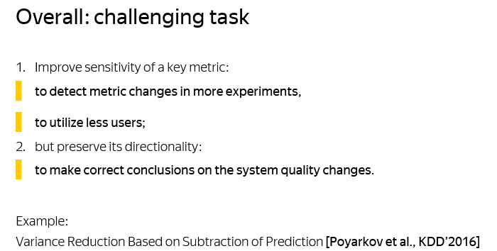
Summing up, we have the following task: to improve the sensitivity of the key metric, but to maintain its focus. Sensitivity, because it will reveal weaker metric changes, and also use fewer users. Both that, and another increases efficiency or productivity of a platform on carrying out experiments. And the focus should be maintained in order to draw the right conclusions about the change in the quality of the system.
Next, I will talk about one of the methods for increasing the sensitivity of a metric, which is used in Yandex, and about which we published an article at the KDD conference in 2016.
This technique is based on subtracting the predictions of the metric value from the metric itself to reduce its variance.

Let's look at the time interval, which is schematically divided into two sub-intervals, for the period of time in which the experiment is conducted, and for a certain period of time before this experiment. Suppose we consider as the key metric the number of sessions held by this user on our site during the experiment.
Let also we have a certain set of indicators, features characterizing the user. For example, the number of sessions of this user that he spent in the pre-experimental period. Similarly, other metrics that we measured in this period can act as features. In addition, we can use some statistical characteristics of the user, for example, gender, age, some other data, if they are available to us.
Finally, let us have some predictor who predicts our key metric based on these indicators. For example, it may be a simple linear model. For example, the simplest and most good predictor is the number of sessions held by the user during the pre-experimental period, if the duration of the pre-experimental period is equal to the duration of the experiment.

The essence of this technique is the following approach: instead of using the metric X, we use the metric Y, which is equal to the metric X, minus the predicted value of the metric X. In our example, this means that instead of looking at the number of sessions in the experiment, we We will look at the change in the number of sessions compared to how much we expected based on our prediction.
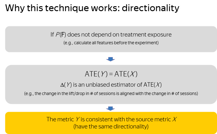
Let's see why this technique works. In fact, we can prove the following theoretical guarantees about our equipment. First, if your predictor does not depend on the experimental output that you are testing or testing. For example, due to the fact that you do not use the factors collected from the user, after the start of the experiment. In this case, you are guaranteed to get the following statement: the average effect of the influence of the new metric is exactly equal to the average effect of the influence of the old metric. This means that the observed change in the metric Y will be an unbiased estimate of the initial metric X. Thus, we guarantee that the metric Y has the same direction as the metric X.

Let us now consider the question of sensitivity. Suppose you are using a predictor that is optimal among machine learning models that are closed with respect to multiplication by a scalar value. Then it is not difficult to prove that the variance of the Y metric will be guaranteed less than the variance of the X metric. This means that the Y metric accurately reduces the variance, or, as we found out, increases the sensitivity.
Thus, we have almost reached the necessary goal, since we have received a new metric that maintains directionality and, in general, can potentially increase sensitivity. Or lower the variance.
Let's understand how much we can lower.
If we additionally require that your predictor be optimal among a class of models that are closed with respect to the addition of a scalar value, then the variance of the metric Y will be exactly equal to the standard deviation of your predictor. This is a very strong and important result. Thus, the degree to which you reduce the variance is exactly the degree to which you improve your predictor. The better you do your predictor, either at the expense of the model, or at the expense of factors, the more you lower the dispersion of metrics and the higher its sensitivity grows.

Summarize. The new metric turned out to be co-directed with the X metric. The new Y metric lowers the variance or increases the sensitivity of the X metric. And besides, you can control the degree of sensitivity increase by improving the quality of the prediction of your original X metric.
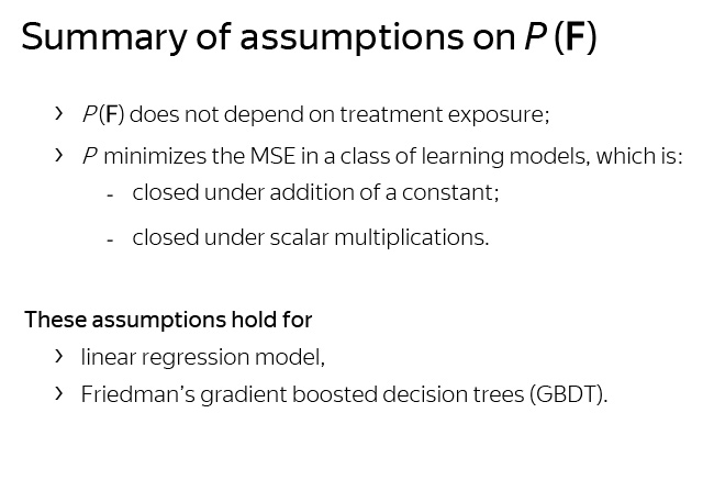
What assumptions have we used for this? First, the predictor’s independence from the experiment, and secondly, the fact that your predictor is optimal from the point of view of the standard deviation in the class of models that are closed with respect to multiplication and the addition of a constant.
In fact, linear models have this property, as well as widely used decision trees, which are constructed by gradient boosting .

We conducted experiments, or rather, studies that considered the number of sessions as a key metric, used 51 factors about the user, in particular, the number of sessions in the pre-experimental period, and the time the user went to the experiment. In addition, we used the 161 AB test as a sample on which we calculated the performance indicators of our approach.
As a result, we managed to achieve the following results. We lowered the variance of the original loyalty metric by 63%, which is equivalent to a threefold reduction in the number of users we need in the experiment in order to obtain T-statistics of the same level as with the original metric.
Finally, we twice as many experiments noticed statistically significant changes. , 2016 .

, , . — , , , . , , . .
, , , , . , , , .

, -, -, WWW, The Web Conference. , , , , ( , QR- — . .).

, - Coursera, . , - . Thanks for attention.
- My report will be about online quality assessment for the effective development of web services. First, I will tell about our team, about what we do.
We in the department of scientific research are engaged in various fields of computer science. This includes data analysis, theoretical foundations of machine learning, processing of natural texts, computer vision and information retrieval, and sometimes it is possible to work on auctions and game theory.
')
Our small department is constantly published at leading conferences in these areas, such as NIPS, ICML, KDD, CVPR, ACL, etc.
Here, only those articles that have been published over the past few years.
In today's report I will talk about one of the areas in which we have been very concentrated in recent years. This is an online assessment of the quality of web services.
Over the past five years, I and my colleagues have been able to make a significant contribution to the development of this subject, we have published 14 articles at leading conferences. One of them received the award for the best article at the leading information search conference in 2015.
Online quality assessment in the development of a web service or product plays a key role in deciding whether to launch new functionality. Let's take a look at how this process works in Yandex.
Dozens of experiments are conducted at any time. An example of the experiment is shown on this slide. We see two options for issuing on the same search query. Next to the results of the issuance of the right there are miniature pictures.
Do you think the right-hand option is better than the left, and improves service? The correct answer will say later.
The slide again shows two options for issuing the same search query. On the right variant there is no factoid.
Do you think the right service option is better than the left one? The correct answer will say later.
The answer to my inquiries strongly depends on what we put into the concept of “improve”. So let's see what is under the hood of AB-testing.
It is useful to recall the key points of support for this process. For each experiment, a certain set of users is allocated that will participate in this experiment. Further, this set is divided randomly into two groups. For example, equally. We define half of the users in group A, and half in group B.
Each of these groups then displays its own version of your website, web service, or product. For example, group A shows the current working version of the product, which is shown to most users, and group B shows the new experimental version of the product, which contains, for example, the new functionality that you want to test.
After the expiration of a certain time, you complete the experiment, for example, in a week or two, and collect some statistics and information about their behavior from all users. For example, it can be one number for each user. This number — for example, the number of user sessions on a site during an experiment — we call the key metric. We aggregate these numbers among all users in each group, and get a number for each of the groups. This is sometimes called an aggregated metric or evaluation criterion. Thus, we get one number for each group. For our example, this is the average number of sessions per user in each group.
Having these two numbers, we take their difference, and compare this difference with zero, in order to understand whether your metric has changed in a positive or negative direction, and also remember how big this difference was.
But this is not enough for you to know. We all know that the division of users into groups is random, the behavior of users is also completely subject to a random process, and therefore the observation of your difference is a certain random variable. Or the implementation of a random variable.
To understand whether the observed difference differs from the possible noise in the data, we apply a statistical test. For example, it may be the well-known Student's t-test.
After that, we decide whether or not the change we are seeing is a consequence of the new functionality we are testing. Or, this observation is just a noise in the data, but in reality your new functionality has no effect on users, at least in terms of this metric.
These two processes lead us to two key properties or metric definitions that a metric should possess. Let's take a closer look at these two properties.
In reality, the observed difference in the average values of the metric X for versions A and B is an unbiased estimate of the average effect of influence, which in turn is also the difference, but already the expected value of the metric X for version A and version B.
Thus, it must always be remembered that the observed delta is a realization of a random variable. Let's imagine that as a result of the experiment we got a delta equal to one percent increase in the number of sessions per user. Is it a lot or a little? This is indicated on the screen as a large segment. This is probably a very large value.
But in order to understand this, you need to find out if we can observe such a delta if the service versions are indistinguishable. The average effect of the effect is zero.
Often this condition is also called the null hypothesis. Here, everything strongly depends on what the distribution of this is. The screen shows two possible distributions. And it is easy to see that if we are dealing with the distribution of blue, then the probability of observing this delta is much less with the null hypothesis than if we are dealing with the distribution of green.
To understand or be sure of the significance of that observation or the observed change, we calculate the probability of observing this delta or more under the condition of the null hypothesis.
To calculate this probability, as a rule, we use the well-known Student's T-test, which is based on T-statistics.
Here is its formula, in the numerator is the delta, and in the denominator there are two more values. The first value is the variance of the metric X for each of the groups. The second is the sample size of each group. The higher the T-statistics module, the more we are confident of the observed change in our delta.
Let's take a closer look at the conditions under which the T-statistics module will be larger. Consider the expression for T-statistics. It depends on three quantities. It is clear that this module of T-statistics will be higher if the numerator is larger, if the experiment greatly changes the metric. Only under this condition will the numerator be larger. For example, if the experiment will shift the metric by 10%, by 20%, by 30%. What other big numbers can we imagine?
But this happens very rarely when your service has been developing and improving for many years. In addition, the size of the change in the experiment depends on the experiment itself, on the functionality that you are testing. If you are testing functionality that has very little impact on users, then the delta will be very small. Therefore, the numerator is not subservient to us. And therefore, if we want to increase T-statistics, then only the denominator depends on us, only we can change it.
The easiest way is to increase the number of users that we use in the experiment. But this method is bad because it reduces the throughput of the experimental platform, which means its efficiency.
An alternative way is to reduce the variance of the metric. Thus, we gradually come to such a concept as the sensitivity of the metric. For simplicity, we assume that this is the average T-statistics module for all experiments. The higher the sensitivity, the weaker changes we can notice in our experiment. Or alternatively, we can use fewer users in the experiment to observe the same changes that we observed before, but at the same level of significance as with the initial number of users.
The main key to increasing sensitivity is reducing the variance of the metric, which I mentioned earlier.
We turn to the second concept - directional metrics.
Consider two metrics: the number of clicks per user during the experiment and the number of sessions per user. It turns out that in this example, the number of clicks per user increased, which indicates a positive effect. Visitors use output better.
In addition, the number of sessions per user has also increased. This means that users began to return to our site more often to solve everyday tasks.
In the second example, we also observe an increase in the number of clicks, since in the right-hand version of the results there is no factoid on the query that the user asked. Therefore, they should search for this answer, going to the site, and make more clicks. Despite this, the right version of the service without a factor leads to a decrease in the number of sessions per user. And in this example, we see that the click metric of user activity conflicts with a more long-term metric that measures user loyalty, and therefore more suitable for an urgent purpose.
In the end, what do we have? The number of clicks is increased, and the number of sessions is reduced in the experiment.
To sum up briefly, we call a good metric one that has a clear interpretation of the directions of its change or direction. And this is a key criterion when choosing a metric. Without this property, it is very difficult for any analyst to make the right conclusion, to make the right decision about the success or failure of the test update or functionality.
Consider some class of user enthusiasm metrics for example. As a rule, two groups of metrics are assigned to this class of metrics. The first group is loyalty metrics, such as the number of sessions per user, the time of his absence, etc. The second group consists of activity metrics. These are such metrics as the number of user clicks, the number of user requests, the time spent on the site, etc.
The first category of metrics has a very good focus. The interpretation of its changes is very transparent and, as a rule, correlates with the company's long-term goals for long-term existence and development.
At the same time, these metrics have very low sensitivity. In our experiments, such metrics are very difficult to move, it is very difficult to invent a new functionality that will significantly increase user loyalty or the number of tasks that they solve in their daily life through our service.
On the contrary, activity metrics have a confused direction, but at the same time they have a very high sensitivity. They are very easy to move. Any experiment that introduces functionality that changes or affects the design, immediately leads to a change in the metric: if users do not like this new functionality, they are forced to study it. Try it, see what happens to it. As a result, they make more or less clicks if they are distracted to perform another action, and the important task is to increase the sensitivity of the loyalty metrics, but at the same time retaining their focus.
Summing up, we have the following task: to improve the sensitivity of the key metric, but to maintain its focus. Sensitivity, because it will reveal weaker metric changes, and also use fewer users. Both that, and another increases efficiency or productivity of a platform on carrying out experiments. And the focus should be maintained in order to draw the right conclusions about the change in the quality of the system.
Next, I will talk about one of the methods for increasing the sensitivity of a metric, which is used in Yandex, and about which we published an article at the KDD conference in 2016.
This technique is based on subtracting the predictions of the metric value from the metric itself to reduce its variance.
Let's look at the time interval, which is schematically divided into two sub-intervals, for the period of time in which the experiment is conducted, and for a certain period of time before this experiment. Suppose we consider as the key metric the number of sessions held by this user on our site during the experiment.
Let also we have a certain set of indicators, features characterizing the user. For example, the number of sessions of this user that he spent in the pre-experimental period. Similarly, other metrics that we measured in this period can act as features. In addition, we can use some statistical characteristics of the user, for example, gender, age, some other data, if they are available to us.
Finally, let us have some predictor who predicts our key metric based on these indicators. For example, it may be a simple linear model. For example, the simplest and most good predictor is the number of sessions held by the user during the pre-experimental period, if the duration of the pre-experimental period is equal to the duration of the experiment.
The essence of this technique is the following approach: instead of using the metric X, we use the metric Y, which is equal to the metric X, minus the predicted value of the metric X. In our example, this means that instead of looking at the number of sessions in the experiment, we We will look at the change in the number of sessions compared to how much we expected based on our prediction.
Let's see why this technique works. In fact, we can prove the following theoretical guarantees about our equipment. First, if your predictor does not depend on the experimental output that you are testing or testing. For example, due to the fact that you do not use the factors collected from the user, after the start of the experiment. In this case, you are guaranteed to get the following statement: the average effect of the influence of the new metric is exactly equal to the average effect of the influence of the old metric. This means that the observed change in the metric Y will be an unbiased estimate of the initial metric X. Thus, we guarantee that the metric Y has the same direction as the metric X.
Let us now consider the question of sensitivity. Suppose you are using a predictor that is optimal among machine learning models that are closed with respect to multiplication by a scalar value. Then it is not difficult to prove that the variance of the Y metric will be guaranteed less than the variance of the X metric. This means that the Y metric accurately reduces the variance, or, as we found out, increases the sensitivity.
Thus, we have almost reached the necessary goal, since we have received a new metric that maintains directionality and, in general, can potentially increase sensitivity. Or lower the variance.
Let's understand how much we can lower.
If we additionally require that your predictor be optimal among a class of models that are closed with respect to the addition of a scalar value, then the variance of the metric Y will be exactly equal to the standard deviation of your predictor. This is a very strong and important result. Thus, the degree to which you reduce the variance is exactly the degree to which you improve your predictor. The better you do your predictor, either at the expense of the model, or at the expense of factors, the more you lower the dispersion of metrics and the higher its sensitivity grows.
Summarize. The new metric turned out to be co-directed with the X metric. The new Y metric lowers the variance or increases the sensitivity of the X metric. And besides, you can control the degree of sensitivity increase by improving the quality of the prediction of your original X metric.
What assumptions have we used for this? First, the predictor’s independence from the experiment, and secondly, the fact that your predictor is optimal from the point of view of the standard deviation in the class of models that are closed with respect to multiplication and the addition of a constant.
In fact, linear models have this property, as well as widely used decision trees, which are constructed by gradient boosting .
We conducted experiments, or rather, studies that considered the number of sessions as a key metric, used 51 factors about the user, in particular, the number of sessions in the pre-experimental period, and the time the user went to the experiment. In addition, we used the 161 AB test as a sample on which we calculated the performance indicators of our approach.
As a result, we managed to achieve the following results. We lowered the variance of the original loyalty metric by 63%, which is equivalent to a threefold reduction in the number of users we need in the experiment in order to obtain T-statistics of the same level as with the original metric.
Finally, we twice as many experiments noticed statistically significant changes. , 2016 .
, , . — , , , . , , . .
, , , , . , , , .
, -, -, WWW, The Web Conference. , , , , ( , QR- — . .).
, - Coursera, . , - . Thanks for attention.
Source: https://habr.com/ru/post/354966/
All Articles