Richard Hamming: Chapter 16. Digital Filters - 3

“The goal of this course is to prepare you for your technical future.”

Hi, Habr. Remember the awesome article "You and your work" (+219, 2394 bookmarks, 377k readings)?



So Hamming (yes, yes, self-checking and self-correcting Hamming codes ) has a whole book based on his lectures. We translate it, because the man is talking.



This book is not just about IT, it is a book about the thinking style of incredibly cool people. “This is not just a charge of positive thinking; it describes the conditions that increase the chances of doing a great job. ”

')

We have already translated 18 (out of 30) chapters. And we are working on the publication "in paper."

Chapter 16. Digital Filters - 3

(For the translation, thanks to Andrey Pakhomov, who responded to my call in the “previous chapter.”) Who wants to help with the translation, layout and publishing of the book - write in a personal or mail magisterludi2016@yandex.ru



And now we are ready to consider the systematic synthesis of non-recursive filters. The method of synthesis of such filters is shown in Figure 16.1 and consists of 6 parts. On the left above the sketch of the filter that you would like to get in the ideal case. It can be a low pass filter, a high pass filter, a bandpass barrier, a band pass filter, a stopper filter, or even a differentiator. For all types of filters, except for the differentiator, they usually strive to obtain a transfer characteristic equal to 0 or 1 at different frequency intervals, while for the differentiator they tend to get iω as a transfer characteristic, because the derivative of the eigenfunction of the filter is equal to







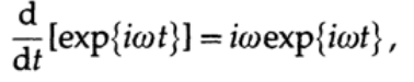
therefore, the desired coefficients are iω.



For the differentiator, a cutoff frequency will most likely be set, because, as you may have noticed, the differentiation increases the amplitude of the signal by multiplying it by ω . In the high-frequency region, where noise is usually located, the transfer function has the highest values ​​(Figure 16.II). Also note in Figure 15.II.







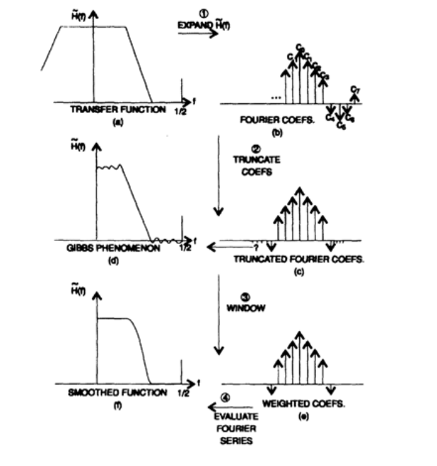
Figure 16.I



The coefficients of the corresponding members of the Fourier series expansion are easily calculated, since the integrands in the expression for their calculation are simple (when there is a derivative, it is possible to use integration in parts). Suppose we presented a series expansion in the form of complex exponentials. Then the filter coefficients are the coefficients of the corresponding members of the series, presented in an exponential form. In the top right corner of Figure 16.I, a symbolic graph of coefficients is presented (of course, coefficients are complex numbers).



At the next stage (presented below in Figure 16.I) we must limit the decomposition in a row to 2N + 1 members (this is similar to using a rectangular window). This limiting the number of members (the right side of the illustration) leads to the Gibbs effect (the left side of the illustration). The coefficients with the window functions imposed on them are presented in the lower right part of the illustration, and the final filter in the lower left part.



The method presented above requires choosing the number of members of the Fourier series (N) and the shape of the window function. If the initial selection of these parameters is not suitable for your task, you select other parameters and try again. This is a trial and error method.



James Frederick Kaiser proposed a method of synthesis, which allows you to simultaneously calculate the number of coefficients of a series, and get a specific window function from a certain family of window functions. In this case, two parameters must be specified: deviation from the ideal filter along the vertical axis (δ) and the width of the transition region between the passband and the suppression bandwidth (ΔF), an example is shown in Figure 16.III.





Figure 16.III



For a band-pass filter, with a given bandwidth f _p and a suppression band f _p , the following sequence of calculations applies:







If the obtained value of N is too large, then you need to stop and revise the design of the filter, otherwise you go to the next step:



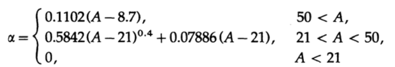The dependence α (A) is presented in graph 16.IV. The initial Fourier series expansion coefficients are given as







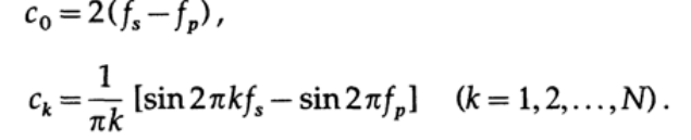
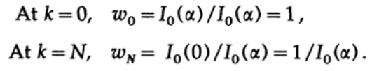
These coefficients should be multiplied by the corresponding weighting factors w _{k of the} window function







Where











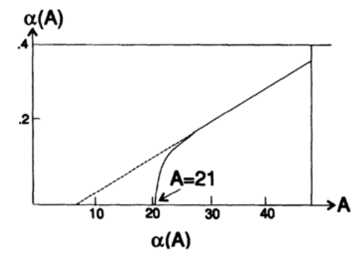
Chart 16.IV



I ₀ ( x ) is the Bessel function of the imaginary argument of zero order. To calculate its value, you need a comparatively few terms, because the series converges quickly due to the square n ! in the denominator.



It is best to calculate the value of I ₀ ( x ) recursively; for a given x, the next member of the series is expressed through the previous as







For a low pass or high pass filter, one of the values ​​of f _p or f _s has limnit possibel for it. For a frequency-rejection filter, the formulas for calculating the coefficients c _k vary slightly.



Let's examine the coefficients of the Kaiser window function, w _k :







If we examine these numbers, we see that for α> 0 they resemble a raised cosine







and the corresponding window function is similar to the windows of Hann and Hamming. For A> 21 there is a “platform”. For A <21, when α = 0, all weighting factors w _k are equal to one and we get a window similar to the Lanczos window. With increasing A, a platform gradually emerges. Thus, the Kaiser window has the same properties as many popular windows, but the specific window that you use is built on the basis of the specified parameters, and not on the basis of prejudice or conjecture.



How did the Kaiser derive these formulas? To some extent by trial and error. Initially, he assumed that he had one gap and he modeled many options on the computer to see the duration of the front ΔF ( the signal front is a signal transition from state 0 (lower level) to 1 (upper level). In this case, there is ie, the width of the transition band between the passband and the attenuation band. ) and the pitch δ. After a fair amount of reflection, the touch of the muse and not having anything defined as a function of A, we note that with increasing A we arrive from the Lanczos window (A <21) to the platform of increasing height, 1 / I ₀ (α). In the ideal case, he wanted to get an elongated spheroidal function, but he noticed that the values ​​obtained by him were precisely approximated by I ₀ ( x ). He built graphs and approximated functions. I asked him how he got 0.4 for the exponent degree. He said that he tried 0.5 at the beginning, but that turned out to be too much, then a value of 0.4, which also perfectly suited, was the next logical choice. This is a good example of the fact that the use of already known knowledge in combination with a computer, as a tool for experiments, leads to very useful results, even in theoretical studies.

Sometimes the Kaiser method fails when there is more than one slice (in fact, the slice is displayed symmetrically and at a negative frequency range) and then the ringing due to different sections will overlap each other and the predicted ringing value will be exceeded. In such a situation, which sometimes does happen, you should simply repeat the synthesis with less stringent restrictions. The entire program can be executed on a small, programmable calculator placed in the hand, for example, TI-59, not to mention a modern PC.



And now let's go back to the final Fourier series. The Fourier functions are remarkable in that they are orthogonal, not only on a continuous interval, but also on a set of individual points equidistant from each other. Therefore, the whole theory remains the same, except that the expansion in a series can have as many members as there are points in the original array. For 2N points, in the general case, only one term for the highest frequency, cosine, is present in the series expansion (since the sine value will be zero at the sampling points). The coefficients are defined as the sum of the data values ​​multiplied by the corresponding Fourier functions. The resulting representation, taking into account the rounding, will reproduce the original data.



The calculation of the decomposition will look like 2N operations of addition and multiplication for each of the 2N values ​​of the original data, that is, something about (2N) ² operations of addition and multiplication. The use of two optimizations: (1) adding and subtracting terms with the same multiplier before performing the multiplication operation and (2) calculating higher frequencies by multiplying lower frequencies resulted in a fast Fourier transform (FFT), which requires N logN operations. Such a reduction in the required computational power has greatly changed the entire field of science and technology - what was previously impossible due to high costs and a long computation time, has become ubiquitous.



And now is the time for another life story. You all have heard about the FFT and the publication of Kuli-Tukey. An FFT is sometimes called a Kuli-Tukey transform or algorithm. Tukey prompted me, in part, the basic ideas of the FFT. At that time, I had an IBM-programmed external punch card calculator (IBM Card Programmed Calculator), and the butterfly operation he had in mind was absolutely not practical on the equipment I had. A few years later, I had a programmable IBM-650 inside, and he reminded me of these optimizations again. All I remembered then was that it was one of Tukey's few bad ideas; I absolutely forgot why she was bad - only because of the limitations of the equipment that I had then. Thus, I did not implement FFT, although the book, which I had already published by that time, shows that I already knew everything that was necessary for that, and could realize FFT very simply!



Moral: if you remember that something cannot be done, then also remember the main reasons why this cannot be done, so that later, when circumstances change, you will not say: “This cannot be done.” Think of my mistake! Could something be more stupid? Fortunately for my ego, this is a common mistake (and I made it more than once), but due to the fact that I got into a mess with CFT, I am now very sensitive to it. I also noticed that others too often make mistakes in the same way — too often! Please remember the story of how foolish I was and what opportunity I missed because of this, and do not make such mistakes yourself. When you decide that something is impossible, do not say again in the future that it is impossible before you do not study in detail why you were right when you said that it was impossible.



Now I have to return to the delicate topic of the power spectrum, which is equal to the sum of the squares of the two coefficients of a given frequency in the real numbers region or the square of the module in the complex domain. An examination of this question will convince you that this value depends only on the signal itself and does not depend on the location of the origin point in time, in contrast to the values ​​of the coefficients, which depend on the location of the origin point. Spectrum plays a very important role in science and technology. It was the spectral lines that opened up the black box of the atomic structure and allowed Bor to look inside. The newer quantum mechanics, which appeared in 1925, changed everything to be a little confident in something, but the spectrum was still the key. We also regularly examine black boxes by examining the dependencies between the spectra of the input and output signals, in order to gain an understanding of their internal structure - note that it is always unique, but in general we get enough information to form new theories.



Let me carefully analyze what we are doing and what we mean by that, because it largely determines what we see in the end. Usually, at least in our imagination, we are dealing with an analog signal. It is usually infinite and we take readings on a time interval of length 2L. This is the same as multiplying a signal by a Lanczos window, or a rectangular window, if you prefer. This means that a convolution of the original signal occurs with the corresponding function of the form (sin x) / x, Figure 16.V - the longer the signal, the narrower the (sinx) / x loops. Each pure spectral line spreads along the corresponding (sinx) / x curve.

Figure 16.V

We then sample at equal time intervals and high frequencies are superimposed on lower frequencies. Obviously, regardless of the order of these two operations — discretization and signal limiting by time — we will get the same result. As I have already mentioned, once, I have carefully worked through the corresponding algebraic transformations to make sure that what should be true from the point of view of the theory is in fact also true in practice.



Then we use PBF, which is just an ingenious and accurate method of obtaining the coefficients of a finite Fourier series. The fact is that when we allow the representation of a signal in the form of a finite Fourier series, we assume that the original function is periodic with a period length equal to exactly the sampling period multiplied by the number of samples taken. We forcibly take all non-harmonic frequencies for harmonics - we forcibly convert a continuous spectrum into a line spectrum. Such mapping is not a local effect, and as you can easily calculate that non-harmonic frequencies are superimposed on all harmonic frequencies, of course, the most on adjacent frequencies, but they also influence on more distant frequencies.



I avoided subtracting the average value — the standard technique from the statistics domain, which is used for convenience or calibration. This technique reduces the amplitude of the zero frequency in the spectrum to zero and introduces a serious discontinuity in the spectrum. If a window function is subsequently used, it will simply spread this gap across adjacent frequencies. During data processing for Tukey, I often used the subtraction of a linear or even quadratic trend, from the flight data of an airplane or a rocket. But the spectrum of the sum of two signals is by no means the sum of the spectra! With the addition of two functions, the individual frequencies are added algebraically, and they can both reinforce each other and completely extinguish, and this will lead to an absolutely false result. A trend line has a big gap at the end (remember that we assume that the functions are periodic), because its coefficients decrease as 1 / k, which is not at all fast. We still partially use them, because we don’t know what to replace them with - and none of those I know has any reasonable arguments against my comments.



But back to the theory. Each spectrum of real noise decreases rather quickly as we strive for an infinite frequency, otherwise it would have infinite energy. But the sampling process itself imposes higher frequencies to lower ones, and such a reduction in bandwidth, as shown in graph 16.VI, tends to lead to a flat spectrum - remember that frequencies add up algebraically. Thus, there is a tendency to observe a flat spectrum for noise, and if the spectrum is flat, then we call this noise white noise. The signal is mainly located in the low frequency region. This statement is valid for several reasons, including the use of oversampling (sampling more often than required by the Nyquist theorem), which allows us to use averaging to reduce the measurement error. Thus, a typical spectrum will look like the one shown in graph 16.VI. Therefore, a low-pass filter is so common for removing noise. No single linear method can separate a signal from noise at the same frequency, but noise outside the signal frequency can be removed by a low-pass filter. Thus, when we use oversampling, we have a chance to remove most of the noise with a low-pass filter.



Remember that we have an implicit limitation that we are dealing with a linear system. Analysis of the stock market using Fourier transforms revealed the presence of extremely white noise in the data, and this was interpreted as the impossibility of forecasting prices on the stock exchange - this is only true if you use simple linear predictors. However, it says nothing about the practical application of nonlinear predictors. Here again we can observe a wide distribution of incorrect interpretation of the results due to the use of a mathematical tool, without an understanding of the fundamentals that underlie it. Little knowledge is a dangerous thing, especially if you have gaps in fundamental knowledge.



I neatly mentioned in the preface to the topic of digital filters that at the time, I thought I did not know anything about them. What I didn’t know then - just because I didn’t know anything about designing recursive digital filters — so much so that I had already created them by that time when I studied the theory of predictor-correctors in relation to the numerical solution of ordinary differential equations. Proof is almost a recursive digital filter!



When I studied how to integrate the system of ordinary differential equations numerically, I was free from stereotypes from the field of digital filters, and I soon realized that a limited input signal, as digital filter experts say, if you integrate it, can cause an unlimited output signal - what they called unstable, but it is absolutely obvious that you should get if you integrate - even a constant value at the input will lead to a linear increase at the output.In fact, when I later encountered the task of landing the trajectory on the moon, where there is no air, and therefore there is no resistance, therefore there is no explicit first derivative in the equation, and I wanted to use such solutions using a suitable formula for numerical integration, I found that I had a quadratic error growth; a small rounding error in the calculation of the acceleration will not be corrected and will lead to a quadratic error in determining the location; error in acceleration leads to a quadratic increase in error in the calculation of the location. This is the root of the problem, in contrast to the Earth, where air resistance plays the role of feedback and corrects the wrong acceleration, and as a result, corrects the error in the location.



Thus, to this day, I have to do with the issue of the stability of digital filters, which means not the exponential growth of the output signal with a limited input signal. At the same time, polynomial growth is allowed, and this is no longer the standard stability criterion inherited from classic analog filters, where if it is not limited, everything will melt in you - in any case, they were never seriously considered as an integration tool.



We will look at this in more detail in the next chapter, which is devoted to recursive filters, which play an important role in integration.



To be continued...



Who wants to help with the translation, layout and publication of the book - write in a personal or mail magisterludi2016@yandex.ru



By the way, we also started the translation of another cool book - “The Dream Machine: The History of Computer Revolution” )