Deep learning using R and mxnet. Part 1. Basics

Content:

1. Installing the mxnet library
2. Used dataset
3. The main function for learning neural networks
4. Iterators
5. Network architecture
6. Initializer
7. Optimizer
8. Callback Functions (Callbacks)
9. Model training
10. Solution of the regression problem on real data

1. Install the mxnet library

A clear installation guide for different versions (CPU / GPU) for different languages ​​and for different devices appeared relatively recently. Preparatory steps such as installing drivers and CUDA / cuDNN were considered in this message , we will not repeat. For Python, by the way, you can collect nothing from source, but simply install with the command pip install mxnet --pre . In a situation where the CPU cores are relatively large, and the RAM is relatively small, when assembling from the source you can face a shortage of memory. In this case, run the build in single-threaded mode: make -j1 .

The library can also be used in code in Julia, Scala, and, suddenly, Perl. And still declared support for work on the Raspberry Pi 3.

2. Used dataset

Create an artificial data set of 10,000 observations ( num_examples ) with two signs ( num_inputs ) and one target variable ( num_outputs ). The true form of the relationship between the predictors and the target variable is set by the function real_fn() , a small Gaussian noise of 0.01 * rnorm(num_examples) added to the values ​​generated using this function:

 num_inputs <- 2 num_outputs <- 1 num_examples <- 10000 real_fn <- function(x) { 2 * x[, 1] - 3.4 * x[, 2] + 4.2 } X <- matrix(rnorm(num_examples * num_inputs), ncol = num_inputs) noise <- 0.01 * rnorm(num_examples) y <- real_fn(X) + noise 

3. The main function for learning neural networks

The learning of neural networks of direct propagation is the responsibility of the mx.model.FeedForward.create() function. The list of parameters it takes is as follows:

• symbol - network architecture as a symbolic description. This is not exactly a graph of computations, since the dimensions of the tensors and the loss function are not given in it, but something similar. The architecture can be drawn using the graph.viz() function, an example will be below;
• X is the matrix / array or iterator of the data used for training. We use arrays when the data is completely stored in memory, and iterators when it does not fit. There are several ready-made iterators (for arrays, for pictures in binary RecordIO format, for csv-files) and the ability to create your own;
• y - values ​​of the target variable. It is set only in the case when X is an array, otherwise the iterator must return everything necessary for learning, including the correct answers;
• ctx - device or list of devices used for training (CPU / GPU). An MXContext object created with mx.cpu() or mx.gpu() ;
• begin.round is the initial count of iterations (epochs) of learning. Changing the default value (1) is necessary only when the model is additionally trained;
• num.round is the number of epochs;
• optimizer - used optimizer, given by name (as a string). The default is stochastic gradient descent ("sgd"). An example of optimizer parameters setting is presented below;
• initializer - an object that specifies the initialization scheme for the model parameters;
• eval.data - a list of the form list(data = R.array, label = R.array) or an iterator with validation data;
• eval.metric is a function for assessing the quality of a model. In addition to the available options, you can also use your own handwritten;
• epoch.end.callback is a function that runs after each training era;
• batch.end.callback - function launched after each batch;
• array.batch.size - batch size when using data as an array. When using iterators, the size of the match in them is specified;
• array.layout - "auto", "colmajor" or "rowmajor" (default is "auto"). Array format: for the rowmajor matrix means that dim(X) = c(nexample, nfeatures) , and colmajor means that dim(X) = c(nfeatures, nexample) . The "rowmajor" format is valid only for matrices. The function mx.io.arrayiter() explicitly requires that the data be converted to the colmajor format, i.e. the matrix will be transposed with respect to the usual view with observations in the rows and signs in the columns;
• kvstore is set as a string and is responsible for the synchronization scheme when training on multiple devices. The default is "local";
• verbose - is responsible for displaying informational messages in the learning process. The default is TRUE;
• arg.params is an optional parameter with a list of NDArray arrays containing model weights;
• aux.params - a similar list of additional parameters;
• input.names - the names of the characters supplied to the input;
• output.names - the names of characters received on output;
• fixed.param - parameters that remain fixed during training (not trained);
• allow.extra.params - allows passing additional parameters that are not required according to the symbolic description of the model. If set to TRUE, if there are such extra parameters in the arg.params and aux.params error will not appear.

4. Iterators

Create an iterator over the data array (matrix):

 batch_size <- 4 train_data <- mx.io.arrayiter(t(X), y, batch.size = batch_size, shuffle = TRUE) 

The function takes as input an array or matrix of attributes (in this case, as already mentioned, the matrix must be transposed), an array with the values ​​of the target variable, and the size of the batch. We also turned on the shuffle of observations with the option shuffle = TRUE . The list of all available iterators looks like this:

 apropos("mx.io") # [1] "mx.io.arrayiter" "mx.io.bucket.iter" # [3] "mx.io.CSVIter" "mx.io.extract" # [5] "mx.io.ImageDetRecordIter" "mx.io.ImageRecordIter" # [7] "mx.io.ImageRecordIter_v1" "mx.io.ImageRecordUInt8Iter" # [9] "mx.io.ImageRecordUInt8Iter_v1" "mx.io.LibSVMIter" 

Now we will not consider any other options or writing our own iterators.

5. Network architecture

The network architecture is described by successive calls of functions of the mx.symbol.* Family, each of which adds abstract representations of the network to the model: fully connected, convolutional, pooling, and others. There are a lot of layers available:

 apropos("mx.symbol") # [1] "is.mx.symbol" # [2] "mx.symbol.abs" # [3] "mx.symbol.Activation" # [4] "mx.symbol.adam_update" # [5] "mx.symbol.add_n" # ..... # [208] "mx.symbol.transpose" # [209] "mx.symbol.trunc" # [210] "mx.symbol.uniform" # [211] "mx.symbol.UpSampling" # [212] "mx.symbol.Variable" # [213] "mx.symbol.where" # [214] "mx.symbol.zeros_like" 

To create a simple linear model that solves the regression problem, use the following code:

 data <- mx.symbol.Variable("data") fc1 <- mx.symbol.FullyConnected(data, num_hidden = 1) linreg <- mx.symbol.LinearRegressionOutput(fc1) 

Draw the resulting architecture:

 graph.viz(linreg) 

6. Initializer

The initializer determines from which initial values ​​the learning of the neural network starts. Since our network is very simple and shallow, it is enough to initialize the weights with random values ​​that have a normal distribution:

 initializer <- mx.init.normal(sd = 0.1) 

The only parameters accepted in this case is the standard deviation. There is also an initializer mx.init.uniform() , the only parameter of which is the limit of the range from which values ​​are generated.

For deep networks, proper initialization of weights is of great importance, so we would use the mx.init.Xavier() option.

This scale initialization scheme was invented in 2010 by Joshua Bengio and Xavier Gloro, after whom the method got its name. Currently used everywhere under different names, for example, in Keras you can find glorot_normal glorot_uniform . The library for Python also contains many other initializers that are not available in the version for R. For example, it is not possible to use the preferred variant of initializing the weights of neurons with the ReLU activation function — Xe initialization.

Parameters of the function mx.init.Xavier() :

• rnd_type is a string specifying the type of distribution ("uniform" or "gaussian") from which weights will be generated;
• factor_type - "avg", "in" or "out" (see below);
• magnitude is a not entirely clear numeric parameter that sets the scale of the weights to be obtained.

If rnd_type = "uniform" and factor_type = "avg" (default), weights will be initialized to random values ​​from the range $$$[- c, c]$where $$$c = \ sqrt {\ frac {3} {0.5 \ cdot (n_ {in} + n_ {out})}}$, $$$n_ {in}$- the number of neurons at the entrance (ie, in the previous layer), $$$n_ {out}$- the number of neurons at the output (ie, in the next layer).

If rnd_type = "uniform" and factor_type = "in , then $$$c = \ sqrt {\ frac {3} {n_ {in}}}$. Similarly, when rnd_type = "uniform" and factor_type = "out" we get $$$c = \ sqrt {\ frac {3} {n_ {out}}}$.

With rnd_type = "gaussian" and factor_type = "avg" weights will be extracted from the normal distribution with standard deviation. $$$\ sqrt {\ frac {3} {0.5 \ cdot (n_ {in} + n_ {out})}}$.

7. Optimizer

The optimizer determines how the network weights are updated. Available options are sgd, rmsprop, adam, adagrad and adadelta. You can create an optimizer with the necessary settings using the general function mx.opt.create() :

 optimizer <- mx.opt.create("sgd", learning.rate = 2e-5, momentum = 0.9) 

To find out about the parameters of each optimizer, which we will pass to the mx.opt.create() call, use the help:

 ?mx.opt.sgd ?mx.opt.rmsprop ?mx.opt.adam ?mx.opt.adagrad ?mx.opt.adadelta 

These functions themselves cannot be called in the usual way (but they can be accessed: mxnet:::mx.opt.adagrad ).

Parameters mx.opt.sgd()

• learning.rate - learning.rate speed;
• momentum - the moment;
• wd is the l2-regularization coefficient (adds a penalty for large weights);
• rescale.grad is the value by which the resulting gradient is multiplied before the weights are updated. Often taken to be 1 / batch_size ;
• clip_gradient - restriction of gradient values ​​by their projection onto the interval $$$[- clip \ _gradient, clip \ _gradient]$;
• lr_scheduler - scheduler changes learning speed.

Parameters mx.opt.rmsprop()

• learning.rate - learning.rate speed;
• gamma1 - attenuation coefficient for a moving average of squares of gradients;
• gamma2 - the moment;
• wd is the l2-regularization coefficient (adds a penalty for large weights);
• rescale.grad is the value by which the resulting gradient is multiplied before the weights are updated. Often taken to be 1 / batch_size ;
• clip_gradient - restriction of gradient values ​​by their projection onto the interval $$$[- clip \ _gradient, clip \ _gradient]$;
• lr_scheduler - scheduler changes learning speed.

Parameters mx.opt.adadelta() :

• rho is the attenuation coefficient for the squares of the gradients and squares of the parameter updates;
• epsilon is a small constant (1e-05) to avoid dividing by 0;
• wd is the l2-regularization coefficient (adds a penalty for large weights);
• rescale.grad is the value by which the resulting gradient is multiplied before the weights are updated. Often taken to be 1 / batch_size ;
• clip_gradient - restriction of gradient values ​​by their projection onto the interval $$$[- clip \ _gradient, clip \ _gradient]$.

Note: for the speed of learning parameter is not provided.

The Adadelta optimizer is similar to RMSprop, but Adadelta makes the second amendment with unit changes and update history storage, and RMSprop simply uses the root of the mean of the squares of the gradients. The following algorithm, Adagrad, uses smoothed versions of mean and rms gradients. You can read more about all this in the book Deep Learning , which is recommended to be read in its entirety.

Parameters mx.opt.adagrad() :

• learning.rate - learning.rate speed;
• epsilon is a small constant (1e-08) to avoid dividing by 0;
• wd is the l2-regularization coefficient (adds a penalty for large weights);
• rescale.grad is the value by which the resulting gradient is multiplied before the weights are updated. Often taken to be 1 / batch_size ;
• clip_gradient - restriction of gradient values ​​by their projection onto the interval $$$[- clip \ _gradient, clip \ _gradient]$;
• lr_scheduler - scheduler changes learning speed.

Parameters mx.opt.adam() :

• learning.rate - learning.rate speed;
• beta1 is the attenuation coefficient for the first moment estimate;
• beta2 is the attenuation coefficient for the second moment estimate;
• epsilon is a small constant (1e-08) to avoid dividing by 0;
• wd is the l2-regularization coefficient (adds a penalty for large weights);
• rescale.grad is the value by which the resulting gradient is multiplied before the weights are updated. Often taken to be 1 / batch_size ;
• clip_gradient - restriction of gradient values ​​by their projection onto the interval $$$[- clip \ _gradient, clip \ _gradient]$;
• lr_scheduler - scheduler changes learning speed.

8. Callback Functions (Callbacks)

We will save the learning history using the appropriate callback function:

 logger <- mx.metric.logger() epoch.end.callback <- mx.callback.log.train.metric( period = 1, #  ,     logger = logger) 

After learning, the logger object will contain information like

 logger$train # [1] 2.322148818 0.318418684 0.044898842 0.011428233 0.009461375 

Other callbacks: mx.callback.early.stop() is responsible for the early stop, mx.callback.log.speedometer() displays the processing speed with a specified frequency, mx.callback.save.checkpoint() saves the model at specified intervals in a file with given prefix.

9. Model training

Learning is started by calling the mx.model.FeedForward.create() function described above:

 model <- mx.model.FeedForward.create( symbol = linreg, X = train_data, ctx = mx.cpu(), num.round = 5, initializer = initializer, optimizer = optimizer, eval.metric = mx.metric.rmse, epoch.end.callback = epoch.end.callback) ## Start training with 1 devices ## [1] Train-rmse=2.39517188021255 ## [2] Train-rmse=0.34100598193831 ## [3] Train-rmse=0.0498822148288494 ## [4] Train-rmse=0.0120600163293274 ## [5] Train-rmse=0.00946668211065784 

Draw the history of learning:

 plot(logger$train, type = "l")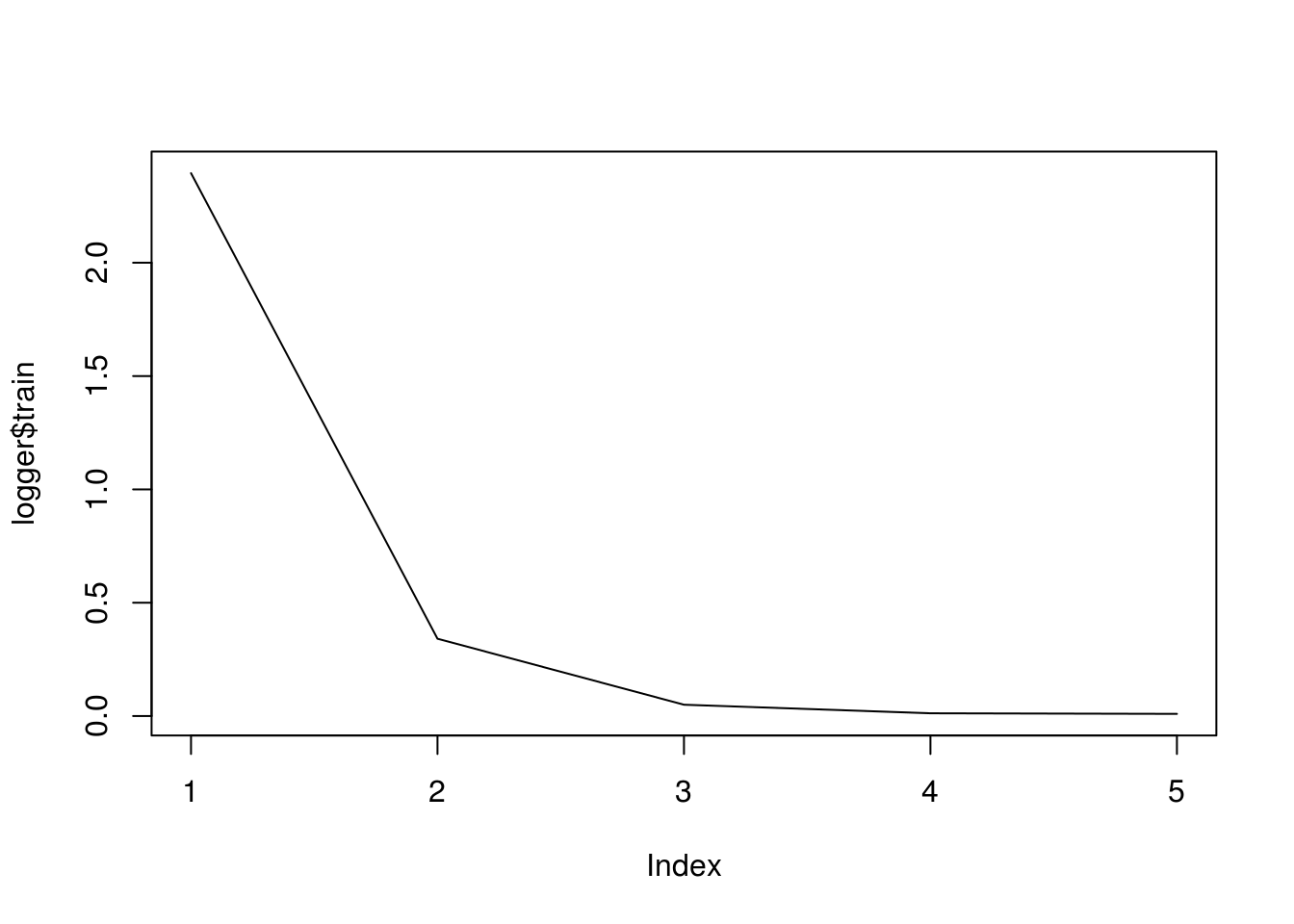 

Check how our model works:

 predict(model, t(X[1:5, ])) y[1:5] ## Warning in mx.model.select.layout.predict(X, model): Auto detect layout input matrix, use colmajor.. ## [,1] [,2] [,3] [,4] [,5] ## [1,] 0.3129134 4.070303 4.975691 8.280487 8.931004 y[1:5] ## [1] 0.3211988 4.0561930 4.9810253 8.2959409 8.9414367 

Everything works, you can move on to a more serious example!

10. Solution of the regression problem on real data

Let us consider the solution of the regression problem on the example of predicting the degree of penetrability (in fact, the speed of passive diffusion) of a substance through a monolayer of cells based on the known properties of this substance (for more details, see here )

The described task is dedicated to the work of the ADME evaluation in drug discovery. 5. Correlation of Caco-2 permeation with simple molecular properties . It contains a table containing the characteristics of 77 substances of various structure, as well as experimental data on the permeability of these substances. It should be noted that the data obtained for the same substance in the course of different experiments can vary considerably. But we will not go into this aspect of the problem, but simply take the data that the authors of the publication worked with.

Load the data using code created by the useful function dump() :

 # df <- read_excel("caco2.xlsx") # dump("df", stdout()) df <- structure(list(name = c("acebutolol", "acebutolol_ester", "acetylsalic_acid", "acyclovir", "alprenolol", "alprenolol ester", "aminopyrin", "artemisinin", "artesunate", "atenolol", "betazolol ester", "betazolol_", "bremazocine", "caffeine", "chloramphenicol", "chlorothiazide", "chlorpromazine", "cimetidine", "clonidine", "corticosterone", "desiprarnine", "dexamethas", "dexamethas_beta_D_glucoside", "dexamethas_beta_D_glucuronide", "diazepam", "dopamine", "doxorubici", "erythromycin", "estradiol", "felodipine", "ganciclovir", "griseofulvin", "hydrochlorothiazide", "hydrocortisone", "ibuprophen", "imipramine", "indomethacin", "labetalol", "mannitol", "meloxicam", "methanol", "methotrexate", "methylscopolamine", "metoprolol", "nadolol", "naproxen", "nevirapine", "nicotine", "olsalazine", "oxprenolol", "oxprenolol ester", "phencyclidine", "Phenytoin", "pindolol", "pirenzepine", "piroxicam", "pnu200603", "practolol", "prazocin", "progesterone", "propranolol", "propranolo_ester", "quinidine", "ranitidine", "salicylic acid", "scopolamine", "sucrose", "sulfasalazine", "telmisartan", "terbutaline", "tesosterone", "timolol", "timolol_ester", "uracil", "urea", "warfarine", "zidovudine"), log_P_eff_exp = c(-5.83, -4.61, -5.06, -6.15, -4.62, -4.47, -4.44, -4.52, -5.4, -6.44, -4.81, -4.52, -5.1, -4.41, -4.69, -6.72, -4.7, -5.89, -4.59, -4.47, -4.67, -4.75, -6.54, -6.12, -4.32, -5.03, -6.8, -5.43, -4.77, -4.64, -6.27, -4.44, -6.06, -4.66, -4.28, -4.85, -4.69, -5.03, -6.21, -4.71, -4.58, -5.92, -6.16, -4.59, -5.41, -4.83, -4.52, -4.71, -6.96, -4.68, -4.51, -4.61, -4.57, -4.78, -6.36, -4.45, -6.25, -6.05, -4.36, -4.37, -4.58, -4.48, -4.69, -6.31, -4.79, -4.93, -5.77, -6.33, -4.82, -6.38, -4.34, -4.85, -4.6, -5.37, -5.34, -4.68, -5.16), log_D = c(-0.09, 1.59, -2.25, -1.8, 1.38, 2.78, 0.63, 2.22, -0.88, -1.81, 0.28, 0.63, 1.66, 0.02, 1.14, -1.15, 1.86, -0.36, 0.78, 1.78, 1.57, 1.89, 0.58, -1.59, 2.58, -0.8, -0.16, 1.26, 2.24, 3.48, -0.87, 2.47, -0.12, 1.48, 0.68, 2.52, 1, 1.24, -2.65, 0.03, -0.7, -2.53, -1.14, 0.51, 0.68, 0.42, 1.81, 0.41, -4.5, 0.45, 1.98, 1.31, 2.26, 0.19, -0.46, -0.07, -4, -1.4, 1.88, 3.48, 1.55, 3.02, 2.04, -0.12, -1.44, 0.21, -3.34, -0.42, 2.41, -1.07, 3.11, 0.03, 1.74, -1.11, -1.64, 0.64, -0.58), rgyr = c(4.64, 5.12, 3.41, 3.37, 3.68, 3.84, 2.97, 2.75, 4.02, 4.58, 5.41, 5.64, 3.43, 2.47, 3.75, 3.11, 3.74, 4.26, 2.79, 3.68, 3.4, 3.6, 5.67, 5.75, 3.28, 2.67, 4.85, 4.99, 3.44, 3.39, 3.7, 3.37, 3.11, 3.72, 3.45, 3.44, 4.16, 4.61, 2.48, 3.34, 0.84, 5.33, 3.67, 4.59, 4.37, 3.38, 2.94, 2.5, 4.62, 3.63, 3.87, 2.91, 2.97, 3.71, 3.55, 3.17, 3.89, 4.02, 4.96, 3.58, 3.63, 4.13, 3.25, 5.13, 2.14, 3.63, 3.49, 5.68, 5.29, 3.15, 3.33, 4.02, 3.98, 1.84, 1.23, 3.45, 3.14), rgyr_d = c(4.51, 5.03, 3.24, 3.23, 3.69, 3.88, 2.97, 2.75, 3.62, 4.52, 5.27, 5.39, 3.38, 2.47, 3.73, 3.11, 3.69, 4.24, 2.79, 3.71, 3.42, 3.66, 5.28, 5.23, 3.28, 2.68, 4.9, 5.01, 3.44, 3.48, 3.48, 3.37, 3.11, 3.79, 3.36, 3.45, 3.16, 4.46, 2.59, 3.36, 0.84, 5.18, 3.74, 4.53, 4.1, 3.43, 2.94, 2.5, 4.37, 3.56, 3.9, 2.91, 2.97, 3.71, 3.4, 3.26, 3.79, 4.09, 4.99, 3.62, 3.53, 4.06, 3.3, 4.57, 2.14, 3.49, 3.54, 5.53, 5.01, 3.15, 3.33, 4.01, 4.13, 1.84, 1.23, 3.5, 3.13), HCPSA = c(82.88, 77.08, 79.38, 120.63, 38.92, 35.53, 20.81, 54.27, 102.05, 86.82, 43.02, 47.14, 49.56, 45.55, 113.73, 138.76, 4.6, 105.44, 30.03, 75.95, 13.8, 90.74, 163.95, 186.88, 25.93, 75.13, 186.78, 138.69, 44.34, 50.34, 139.45, 67.55, 142.85, 93.37, 39.86, 3.56, 67.13, 93.29, 127.46, 93.21, 25.64, 204.96, 51.29, 44.88, 86.73, 76.98, 36.68, 15.1, 144.08, 48.62, 49.58, 1.49, 65.63, 52.8, 59.71, 99.19, 69.89, 64.79, 86.76, 38.1, 40.42, 36.21, 43.77, 105.15, 61.71, 57.35, 187.69, 133.67, 55.48, 79.52, 42.35, 100.74, 96.25, 66.72, 82.72, 59.47, 96.33), TPSA = c(87.66, 93.73, 89.9, 114.76, 41.49, 47.56, 26.79, 53.99, 100.52, 84.58, 50.72, 56.79, 43.7, 58.44, 115.38, 118.69, 6.48, 88.89, 36.42, 74.6, 15.27, 94.83, 173.98, 191.05, 32.67, 66.48, 206.07, 193.91, 40.46, 64.63, 134.99, 71.06, 118.36, 94.83, 37.3, 6.48, 68.53, 95.58, 121.38, 99.6, 20.23, 210.54, 59.06, 50.72, 81.95, 46.53, 58.12, 16.13, 139.78, 50.72, 56.79, 3.24, 58.2, 57.28, 68.78, 99.6, 91.44, 70.59, 106.95, 34.14, 41.49, 47.56, 45.59, 86.26, 57.53, 62.3, 189.53, 141.31, 72.94, 72.72, 37.3, 79.74, 85.81, 58.2, 69.11, 63.6, 103.59), N_rotb = c(0.31, 0.29, 0.23, 0.21, 0.29, 0.27, 0.17, 0.07, 0.16, 0.29, 0.27, 0.26, 0.15, 0.12, 0.28, 0.08, 0.14, 0.33, 0.08, 0.1, 0.11, 0.13, 0.17, 0.17, 0.06, 0.23, 0.18, 0.21, 0.06, 0.22, 0.25, 0.16, 0.08, 0.12, 0.24, 0.13, 0.19, 0.24, 0.44, 0.16, 0.2, 0.26, 0.16, 0.3, 0.24, 0.19, 0.05, 0.07, 0.27, 0.31, 0.29, 0.04, 0.06, 0.23, 0.08, 0.13, 0.15, 0.29, 0.15, 0.07, 0.22, 0.22, 0.14, 0.33, 0.19, 0.15, 0.28, 0.2, 0.15, 0.29, 0.06, 0.24, 0.23, 0, 0.29, 0.15, 0.18), log_P_eff_calc = c(-5.3, -4.89, -5.77, -5.91, -4.58, -4.39, -4.63, -4.47, -5.64, -5.85, -5.2, -5.13, -4.57, -4.89, -5.11, -5.87, -4.38, -5.55, -4.69, -4.78, -4.46, -4.77, -5.83, -6.55, -4.45, -5.27, -6, -5.13, -4.57, -4.44, -5.79, -4.59, -5.62, -4.94, -4.78, -4.28, -5, -5.09, -5.87, -5.27, -4.67, -6.79, -5.37, -4.99, -5.15, -5.09, -4.49, -4.65, -6.97, -4.84, -4.45, -4.42, -4.6, -5.02, -5.3, -5.31, -6.37, -5.5, -5.05, -4.54, -4.57, -4.5, -4.46, -5.6, -5.29, -5.07, -6.56, -6.06, -4.85, -5.36, -4.53, -5.35, -4.82, -5.23, -5.29, -4.95, -5.43), residuals = c(-0.53, 0.28, 0.71, -0.24, -0.04, -0.08, 0.19, -0.05, 0.24, -0.59, 0.39, 0.61, -0.53, 0.48, 0.42, -0.85, -0.32, -0.34, 0.1, 0.31, -0.21, 0.02, -0.71, 0.43, 0.13, 0.24, -0.8, -0.3, -0.2, -0.2, -0.48, 0.15, -0.44, 0.28, 0.5, -0.57, 0.31, 0.06, -0.34, 0.56, 0.09, 0.87, -0.79, 0.4, -0.26, 0.26, -0.03, -0.06, 0.01, 0.16, -0.06, -0.19, 0.03, 0.24, -1.06, 0.86, 0.12, -0.55, 0.69, 0.17, -0.01, 0.02, -0.23, -0.71, 0.5, 0.14, 0.79, -0.27, 0.03, -1.02, 0.19, 0.5, 0.22, -0.14, -0.05, 0.27, 0.27)), row.names = c(NA, -77L), class = c("tbl_df", "tbl", "data.frame" )) 

The target variable is log_P_eff_exp - the logarithm of the diffusion rate (measured in cm / s).

List of predictors:

• log_D - distribution coefficient at pH = 7.4;
• rgyr is the radius of gyration;
• rgyr_d is the dynamic radius of gyration;
• HCPSA is the area of ​​a highly charged polar surface ;
• TPSA - topological area of ​​the polar surface;
• N_rotb - the number of turning links .

Consider the predictor distributions, as well as their pairwise correlations:

 GGally::ggpairs(df, columns = c(3:8), diag = list(continuous = "barDiag")) 

The variables rgyr and rgyr_d , as well as HCPSA and TPSA predictably strongly correlate, since in both cases the pairs of variables are different ways of calculating the same physical quantity.

Let's teach the same neural network as in the previous example. , .

 set.seed(42) train_ind <- sample(1:77, 60) x_train <- as.matrix(df[train_ind, 2:8]) y_train <- unlist(df[train_ind, 9]) x_val <- as.matrix(df[-train_ind, 2:8]) y_val <- unlist(df[-train_ind, 9]) data <- mx.symbol.Variable("data") fc1 <- mx.symbol.FullyConnected(data, num_hidden = 1) linreg <- mx.symbol.LinearRegressionOutput(fc1) initializer <- mx.init.normal(sd = 0.1) optimizer <- mx.opt.create("sgd", learning.rate = 1e-6, momentum = 0.9) logger <- mx.metric.logger() epoch.end.callback <- mx.callback.log.train.metric( period = 4, #  ,     logger = logger) n_epoch <- 20 model <- mx.model.FeedForward.create( symbol = linreg, X = x_train, y = y_train, ctx = mx.cpu(), num.round = n_epoch, initializer = initializer, optimizer = optimizer, eval.data = list(data = x_val, label = y_val), eval.metric = mx.metric.rmse, array.batch.size = 15, epoch.end.callback = epoch.end.callback) 

, RMSE :

 rmse_log <- data.frame(RMSE = c(logger$train, logger$eval), dataset = c(rep("train", length(logger$train)), rep("val", length(logger$eval))), epoch = 1:n_epoch) library(ggplot2) ggplot(rmse_log, aes(epoch, RMSE, group = dataset, colour = dataset)) + geom_point() + geom_line()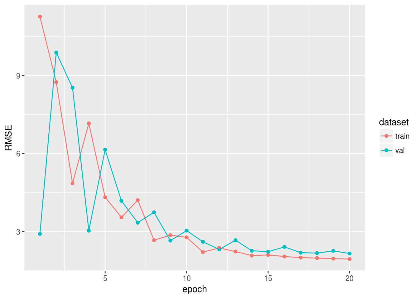 

In the next report, we will solve the classification problem on real data, and also consider other quality metrics and the use of an early stop.