Richard Hamming: Chapter 15. Digital Filters - 2

“The goal of this course is to prepare you for your technical future.”

Hi, Habr. Remember the awesome article "You and your work" (+219, 2372 bookmarks, 375k readings)?



So Hamming (yes, yes, self-checking and self-correcting Hamming codes ) has a whole book based on his lectures. We translate it, because the man is talking.



This book is not just about IT, it is a book about the thinking style of incredibly cool people. “This is not just a charge of positive thinking; it describes the conditions that increase the chances of doing a great job. ”

')

We have already translated 17 (out of 30) chapters. And we are working on the publication "in paper."

Chapter 15. Digital Filters - 2

(For the translation, thanks to Andrey Pakhomov, who responded to my call in the “previous chapter.”) Who wants to help with the translation - write in a personal or mail magisterludi2016@yandex.ru



When digital filters first appeared, they were considered as a kind of classic analog filters; people did not consider them as something fundamentally new and different from the existing one. Exactly the same error was spread during the appearance of the first computers. I was told tirelessly that a computer is just a quick calculator, and everything that a machine can calculate can be calculated by a person. This statement simply ignores the differences in speed, accuracy, reliability, and cost between manual and machine labor. Usually, changing an amount by an order of magnitude (10 times) leads to fundamental changes, and computers are many, many times faster than manual calculations. Those who claimed that there was no difference did not do anything meaningful for the development of computers. Those who made a significant contribution saw something new in computers, something that should be evaluated in a completely different way, and not just like the same old calculators, it can only be a little faster.



This is a common, infinitely repeatable error. People always want to think that something new is something very similar to the old. They like to leave their minds in the comfort zone, as well as the body - so they protect themselves from the possibility of making any significant contribution to new industries that arise right under their nose. Not everything that is called new is in fact, and in some cases it is difficult to determine whether something is truly new. However, the general installation “There is nothing new here” is stupid. When something is called new, do not rush to think that it is just an improvement of something old — it can be a great opportunity for you to do something significant. But again, this may not really be anything new.



The first digital filter, which I used in the times of primitive computers, performed first threefold anti-aliasing, and then fivefold. Recalling the smoothing formula, the transfer characteristic with triple smoothing is defined as







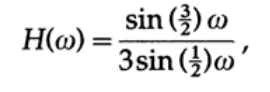
and can be easily drawn (Figure 15.I). The transfer characteristic in the case of a fivefold smoothing looks exactly the same, only 3/2 is replaced by 5/2, and can also be easily drawn (figure 15.I). For two consecutive filters, the total transfer characteristic is obviously the product of their transfer characteristics (each multiplies the input signal — its own function — by the transfer characteristic for the corresponding frequency). You will see three zeros in the interval, and the final value will be 1/15. Further research will show you that the upper half of the frequencies were rather well filtered by a simple computer program that counted the sum of three numbers, then the sum of 5 numbers and this is a common computer practice to transfer all division operations to the end and replace with one multiplication - multiply the result by 1 /15.



Now you probably wondered exactly how a digital filter removes certain frequencies from an array of numbers - even those students who have completed a course on digital filters may not fully understand how it works.







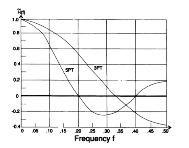
Figure 15.I.



Therefore, I suggest you synthesize a simple filter with only 2 coefficients — that is why I can impose exactly two restrictions on the transfer function. In theory, we use cyclic frequency, but in practice we use frequency. These two quantities are related as follows:







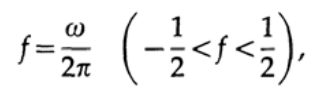
Let us formulate the restrictions for our filter as follows: suppose for the frequency f = 1/6 the value of the transfer characteristic of the filter is 1 (this frequency must pass through the filter without changes), and for the frequency f = 1/3 the value of the transfer characteristic must be zero.



My simple filter looks like this.







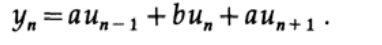
where a and b are parameters whose values ​​we will try to determine.



Substituting exp (2pifn) into the eigenfunction, we get the transfer characteristic.



Substitute n = 0 for convenience and we obtain the following system of equations:







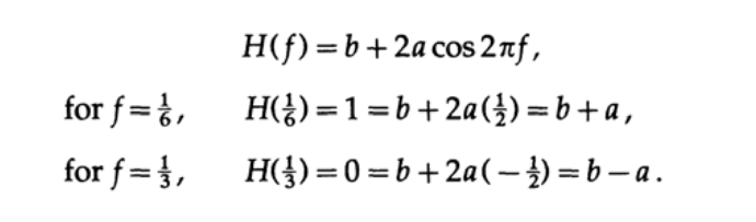
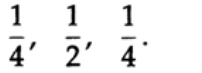
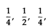
This system of equations has the solution a = b = 1/2, and the desired smoothing filter is a simple expression







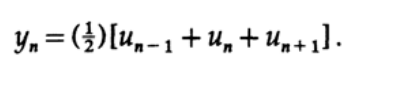
In other words, the value at the output of the filter is equal to the sum of three consecutive values ​​at the input of the filter, divided by three. The value at the output of the filter is located opposite the central value of the input data.



Let's feed some test data to the input of the filter. As a signal transmitted at a frequency of 1/6, we will use the values ​​of the cosine function of the same frequency, taken at regular intervals (n = 0, 1, 2, ...). Similarly, we simulate the signal values ​​at the frequency 1/3. The value of the signal applied to the filter input at a certain point in time will be equal to the sum of the values ​​of these signals at the same time point.







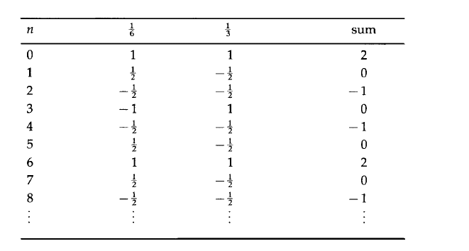
And now let's pass this signal through our filter. According to the obtained filter formula, we will take the sum of three consecutive numbers in a column and divide it by 2. Doing this operation on the first column, you will see that every time the filter is shifted down one line in the table, it reproduces the function given to the input ( multiplied by 1). Pass the second column through the filter, and you will see that the output value is always zero, or the input function value multiplied by its own value 0. The third column filtering, which is the sum of the first two, should skip the first frequency and stop the second one. That is, after filtering the third column, you will receive the first column. You can try to input a signal with a frequency equal to zero. In this case, you should get exactly 3/2 for each value. If you try the frequency f = 1/4, you should get the input values ​​multiplied by ½ (the value of the transfer characteristic for f = 1/2).



You just saw the digital filter in action. The filter decomposes the input signal into all its component frequencies, multiplies each frequency by its own eigenvalue (transfer characteristic), and then sums them together to get the value at the output. All this makes one simple linear filter formula!

Let's go back to the problem of filter synthesis. Often we want to get a transfer characteristic with a sharp drop between the frequencies that it transmits unchanged (with its own value of 1) and the frequencies that it stops (with its own value of 0). As you know, such a function with a discontinuity can be expanded into a Fourier series, but this series will contain an infinite number of members. Despite this, we have a limited number of such members, if we want to get a practically realizable filter; 2k + 1 terms in the smoothing filter allow only k + 1 free coefficients to be obtained, so only k + 1 normal conditions can be imposed on the appropriate sum of cosines.



If we simply decompose the desired transfer function into a series of cosines, and then reduce the number of terms in it, then we obtain an approximation of the transfer characteristic using the least squares method. But at the points of discontinuity, approximation by the least squares method does not lead to the results that you can expect.

In order to understand what we will see at break points, we must investigate the Gibbs effect. To begin with, we recall the theorem: if a series of continuous functions converges uniformly on an interval, then the sum of the series is continuous on this interval. But the function that we approximate is not continuous - it has a jump (discontinuity) at the point of separation of the passband and the stopband. It does not matter how many members of the series we will use. Since there cannot be a uniform convergence here, we can expect to see a significant surge in the vicinity of a singular point (discontinuity point). As the number of row members increases, the magnitude of the burst will not tend to zero.



Here is another bike. Michelson, known for his Michelson-Morley experiment, built an analog device that allows you to determine Fourier expansion coefficients up to 75 members. This device also made it possible to go from coefficients to function. When Michelson restored the function according to the coefficients of the Fourier series, he found a surge and asked local mathematicians why this was happening.







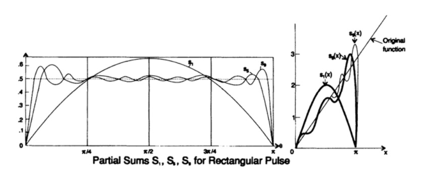
Chart 15.2



They all said that the reason for his equipment - and this despite the fact that he was widely known as a pedantic experimenter. And only Gibbs, from Yale University, listened and studied the question. The simplest and straightforward approach is to decompose a regular function with a discontinuity, say in a Fourier series with a finite number of members, reassemble the original function and find the point of the first maximum and the value of the function at this point.







On chart 15.2, you can detect a surge at 0.0849, or a surge of 8.949%, in the limit with the number of members of the Fourier series tending to infinity. Many people had the opportunity to discover (in fact, rediscover) the Gibbs effect, but it was Gibbs who made the effort. This is one more confirmation of the fact that I constantly affirm that there are plenty of opportunities around us, and only a few people realize them. As Pasteur said, "Fortune smiles only to those who are ready for this." This time, a person became famous, who turned out to be ready to hear a first-class scientist and help him solve his problem.



I noted that this effect was rediscovered. Exactly. In the Cauchy textbook of 1850, we can find two contradictory statements: (1) convergent series of continuous functions converge to a continuous function and (2) expansion in a Fourier series of a function with discontinuities. Some people understood the question and found that it is necessary to introduce the concept of uniform convergence. Just so, the Gibbs effect manifests itself in the decomposition into a series of any continuous functions, and not only for Fourier series. This fact was known to individuals, but did not find wide application. In the general case, when decomposing a series of orthogonal functions, the size of the burst depends on where the discontinuity of the function is located. This distinguishes the Fourier functions from other orthogonal functions; for the Fourier expansion, the magnitude of the burst does not depend on where the discontinuity is located.



It is necessary to remind you of another property of the Fourier series. If the function exists, then the coefficients decrease as 1 / n. If the function is continuous (the values ​​from the two ends of the extremum are the same and the derivative exists at this point, then the coefficients decrease as 1 / n ^2. If the first derivative is continuous and the second derivative exists, then they decrease as 1 / n ^3. Thus, the rate of convergence the series is determined by the function located in along the axis of the real numbers - which is not true for the Taylor series, whose convergence is determined by special points that can lie in the complex plane.



Now back to the design of our digital smoothing filter using the Fourier transform to get the first members of the series. As we see, the least squares approximation has problems at singular points - disgusting bursts in the transfer function consisting of a finite number of terms, and it does not matter how many members of the series we will use.







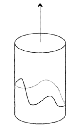
Figure 15.3



To begin with, consider the Lanczos window (it is also called the "rectangular window" or "rectangular function"), which allows you to remove the splash. Lanczos reasoned as follows: “if we average the value of the output function on an interval of length equal to the period of the function with the highest frequency present in the output signal, then this will greatly reduce the ringing”. To consider this in more detail, we take the first N harmonics of the expansion in a Fourier series and take the integral on the symmetric interval around the point t with a length of 1 / N of the entire interval. We write the integral for averaging as







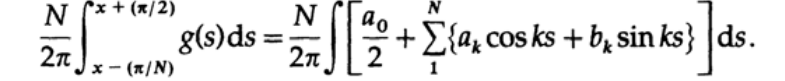
Now let's take the integral:







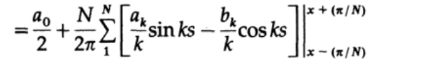
apply the formula of the difference of sines and cosines for the boundaries of the integration interval:







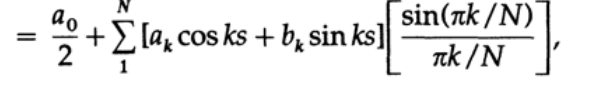
And we get the initial coefficients multiplied by the so-called sigma factors:







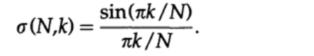
Consideration of the sequence of such numbers as a function of k (N is fixed and equal to the number of taken harmonics of the Fourier series expansion) shows that for k = 1 sigma, the factor is one, and with increasing k, sigma factors decrease to zero with k = N. That is, they are another example of a window function. The result of applying the Lanczos window is to reduce the burst to 0.01189 (7 times) and the first minimum to 0.00473 (10 times), which is a significant, but not complete decrease in the Gibbs effect.



But back to my adventures in this area. I knew, like you, that at the points of discontinuity, expansion in a Fourier series with a finite number of terms is equal to the average of the two limits taken to the left and right of the discontinuity point. Speaking about the finite, discrete case, I concluded that instead of taking the unit in the passband and zero in the attenuation band, use ½ as an intermediate value.



And so, the transfer characteristic began to look like







and now has an extra multiplier (back to frequency notation again)







The N + 1 in the sine terms of the series has passed to N, as well as the denominator N + 1 has moved to N. Obviously, this transfer characteristic for a low pass filter is better than that of Lanczos because it decays at the Nyquist frequency and additionally suppresses all overlying frequencies . I looked at books on trigonometric series and only in one of them - Zygmund's two-volume book - I found mention of such a series: there it was called a modified series. It is not necessary that if I spent more time studying the theory, I would get an outstanding result. Having received such a modification of the expansion into a series on my own, I naturally continued to reflect on further changes in the coefficients of the Fourier series (I still had to figure out which coefficients and how to change), I could get the best result. In short, I understood more clearly what “window functions” are and slowly approached a more detailed study of their capabilities.



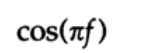
There is a third approach to the Gibbs phenomenon through the union of Fourier series. Let g (x) be (we have a good reason to use the neutral variable x in this case):







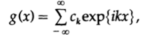
and the other function will be







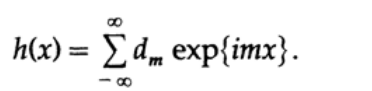
The sum and difference of g (x) and h (x) will obviously be equal to the corresponding series with the sum and difference of the coefficients.



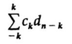
The work is different. Obviously, we again obtain the sum of the exponentials, and by defining n = k + m we obtain the indicated coefficients:







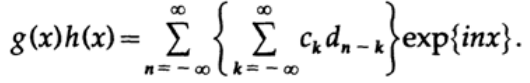
The coefficient for exp {inx}, which is the sum of the terms, is called the convolution of the original coefficient arrays.



In the case when in the array c _k only a few coefficients are not zero, take for example a branch with symmetry about 0, we get the following expression for the coefficient:







And this is the original definition of a digital filter! Thus, a filter is a convolution of two arrays, which in turn is simply a multiplication of the corresponding functions. Multiplication on the one hand of equality and convolution on the other.



As an example of using this observation in practice, let us present a fairly common case: there is an infinite array of data, but we can record only a finite number of values ​​(for example, turning the telescope on and off while observing the stars). Such a function u _n is observed through a rectangular window, where all values ​​outside 2N + 1 are equal to zero. In other words, at the moments of observation, the window function is equal to 1, and the rest of the time is 0.



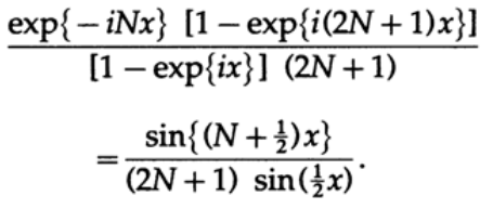
When we try to calculate the Fourier series of the original array by the recorded values, we must calculate the convolution of the coefficients of the original array and the window function:







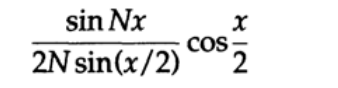
As a rule, we want to get a window area of ​​one, so we must divide by (2N + 1). The resulting array is a geometric progression with the first term exp {-iNx} and the denominator of the progression exp {ix}.







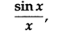
At x = 0, the value of the expression is 1, in other cases, the value of the expression quickly fluctuates due to the sine in the numerator and slowly decays due to an increase in the value of the sine in the denominator (x belongs to the interval (-π, + π). Thus, we obtained a typical diffraction pattern of optics .



In the case of a continuous signal before sampling, the situation develops in a similar way, only a rectangular window through which we observe the signal has a general form of transformation (ignoring all the details):







its convolution with a step function (discontinuity) will lead to the appearance of the Gibbs effect (Figure 15.II). Thus, we saw bursts due to the Gibbs effect in a different light.



Some fairly complex trigonometric transformations will convince you that both the discretization of a function and the subsequent limitation of the observation interval, and the limitation of the observation interval followed by discretization will lead you to the same result. The theory will tell you the same thing.



Simply changing the two external coefficients of a discrete Lanczos window from 1 to ½ leads to a better window function. -, , , - – .







, - , , .



:







. . , , , - . , , , , , .



, , , . , . , -

« »







– « » ( 15.IV),











15.4



N, , . , . . , , , , , .



, . : « , , , , , , ». , , . , - . «»! !



, , , . , , . , , . – . . , , – . . , , .



, , , . , , – , ! , !





To be continued...



Who wants to help with the translation - write in a personal or mail magisterludi2016@yandex.ru



, — «The Dream Machine: » )