Detection of body parts using deep neural networks
Hi, Habr!
Today I will tell you about one of the methods for solving the pose estimation problem. The task is to detect body parts in photos, and the method is called DeepPose . This algorithm was proposed by the guys from Google back in 2014. It would seem, not so long ago, but not for the field of deep learning. Since then, many new and more advanced solutions have appeared, but for a full understanding it is necessary to get acquainted with the origins.
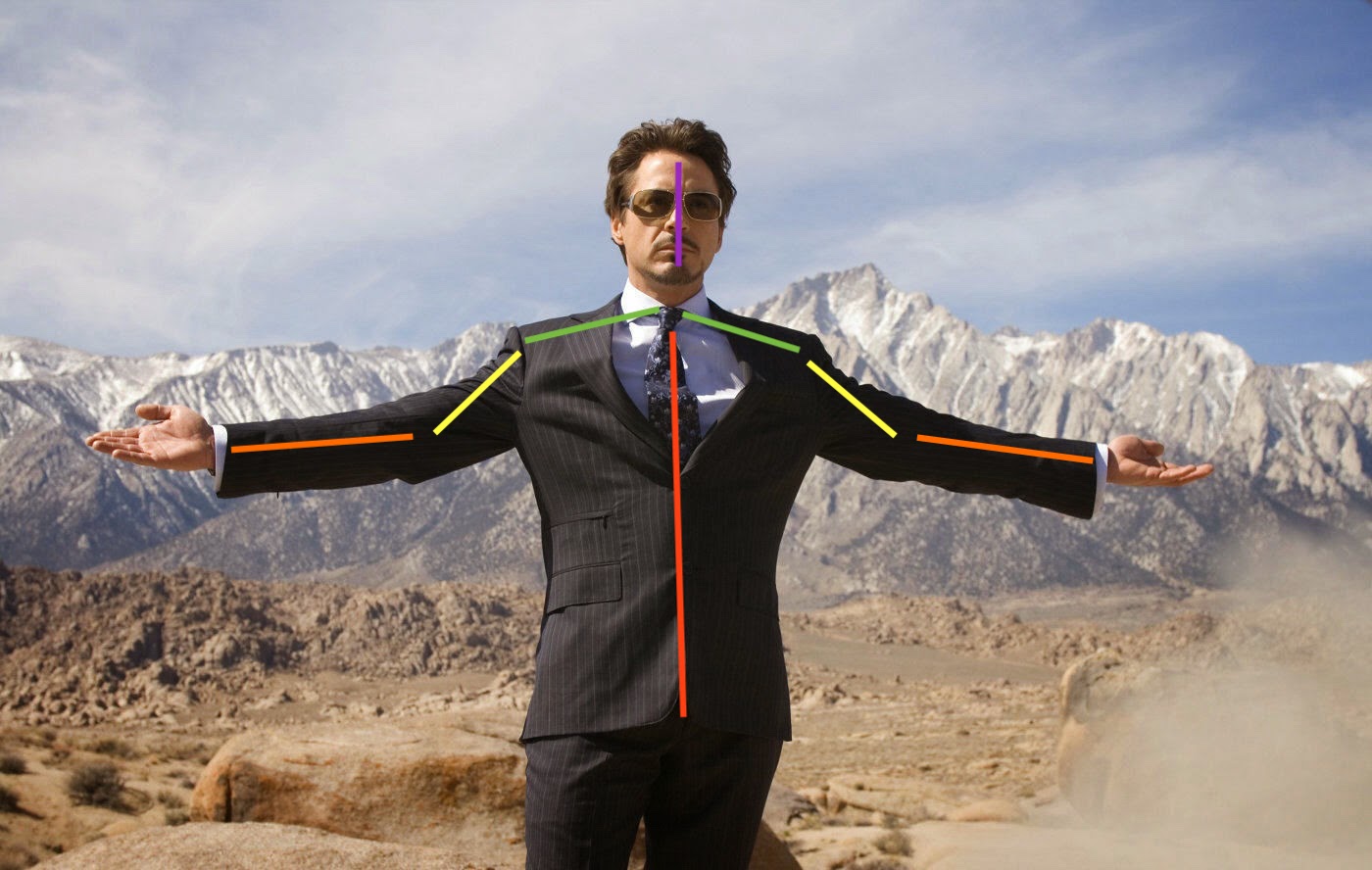
Let's first briefly about the formulation of the problem. You have photos in which a person is present (one or more), and you want to mark out body parts on these photos. That is, to say where the hands, legs, head, and so on.
')
Where would such a markup be useful? The first thing that comes to mind is video games. You can play your favorite RPG, swinging a virtual sword, rather than clicking the mouse. To do this, it is enough to be able only to recognize the movements of your hands.
Of course, there are much more practical applications. For example, tracking how customers in a store put goods in their cart, and sometimes put them back on the shelf. Then you can automatically track what the visitor bought, and the need for cash registers will disappear. Amazon has already implemented this idea in its AmazonGo stores.
I think the above examples of use are already interesting enough to take on the task. However, if you have original ideas of where else you can apply the concepts discussed, feel free to write them in the comments.
How to solve this problem without neural networks? You can imagine a human skeleton in the form of a graph, where the vertices will be the joints, and the ribs will be the bones. And then come up with some mathematical model that will describe the likelihood of a joint in a particular location of the image, and will also take into account how realistic these joints are located relative to each other. For example, so that your left heel is not on your right shoulder. Although, I do not exclude that there are people capable of it.
One of the options such a mat. The model was implemented in the pictorial structures model framework as early as 1973.
But you can approach the solution of the problem in a less cunning way. When we are given a new picture, let's just search in our original set of tagged pictures that are similar and display its markup. If we initially have not very many different postures of people, then this method is unlikely to take off, but, you see, it is not difficult to implement it. To search for similar images there are usually used classical methods for extracting features from the image processing area: HOG , Fourier descriptor , SIFT, and others.
There are other classic approaches, but here I will not dwell on them and move on to the main part of the post.
As you might have guessed, the authors of the article DeepPose (Alexander Toshev, Christian Szegedy) offered their solution using deep neural networks. They decided to consider this problem as a regression problem. That is, for each joint in the photo you need to determine its coordinates.
Next, I will continue the description of the model in a more formal language. But for this you need to enter some notation. For convenience, I will stick to the notations of the authors.
Denote the input image as and vector poses as where contains coordinates th joint. That is, we are now representing the human skeleton as a graph from vertices. Then the marked-up image will be denoted as where - our training dataset.
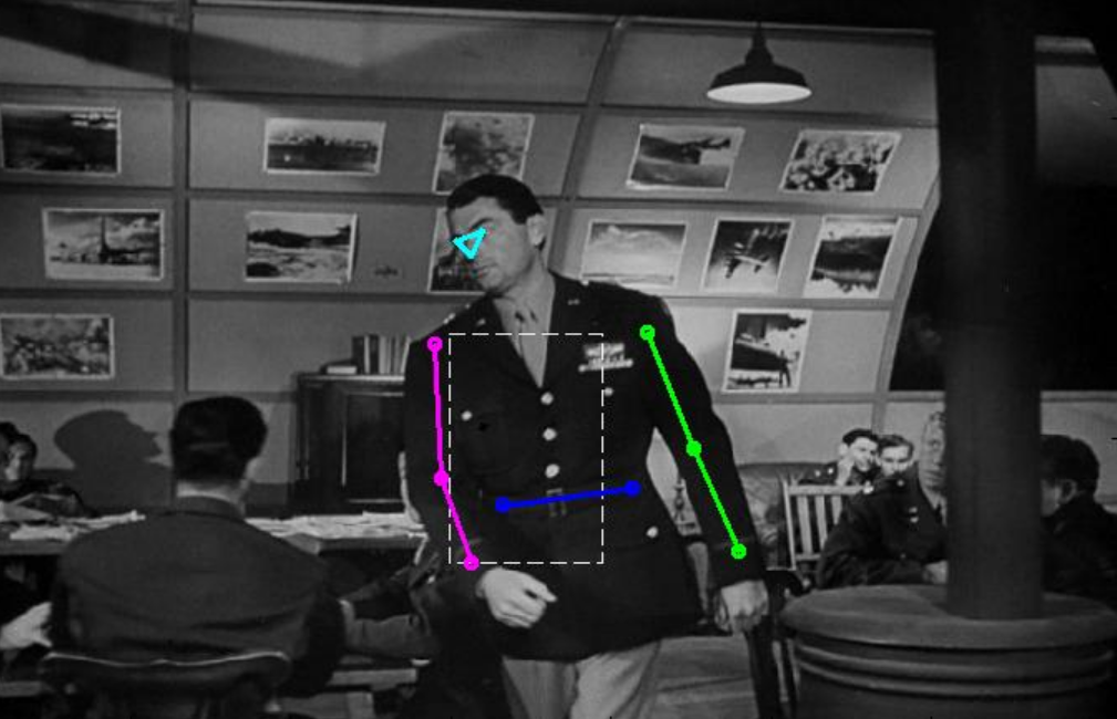
Since the pictures can be of different sizes, as well as the people in the photographs can be represented at different scales and be in different parts of the frame, it was decided to use bounding boxes ( AABB ), which would select the desired image area (the entire human body or more detailed if we are interested in a specific part of the body). Regarding the center of such a region, one can also consider the normalized coordinates of interior points. In the most trivial case, the area can be the entire source image.
Denote the bounding box with the center at wide and tall three numbers .
Then the normalized pose vector regarding the area can be written like this
That is, we subtracted the center of the desired region from all coordinates, and then divided coordinate to the width of the rectangle, and Coordinate height. Now all coordinates began to lie in the interval from before inclusive.
Finally, for denote clipping the original image bounding area . The trivial box, which is equal to the original picture, we denote by .
If we now take the function ( - input image - model parameters, - the number of defined joints), which gives the normalized pose vector, then the pose vector in the original coordinates .
As a function we have a neural network whose weights are described . That is, we feed a three-channel image of a fixed size to the input, and at the output we get joint coordinate pairs:
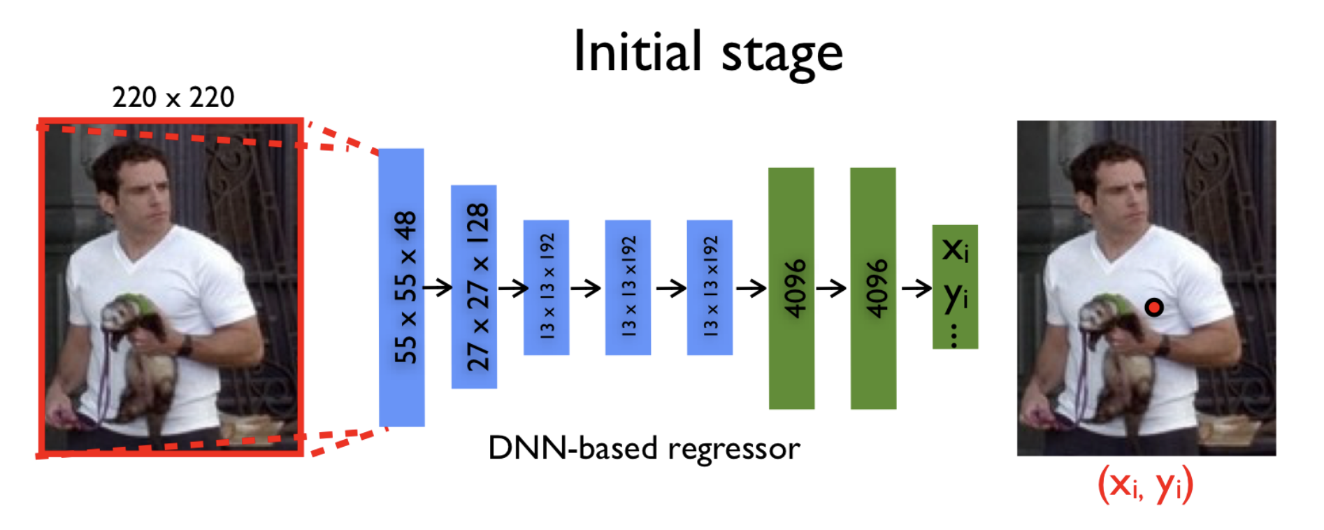
It would seem that already at this stage we can take some deep neural network (for example, AlexNet, which performed well on the task of image classification, winning the ImageNet competition in 2012) and train it in regression. We will find such model parameters to minimize the sum of squares of deviations of the predicted coordinates from the true ones. That is the ideal parameters . Thus, we are trying to restore the original coordinates of the joints independently of each other.
However, since the input to the neural network takes a picture of a fixed size (namely, pixels), some of the information is lost if the picture was originally in the best resolution. Therefore, the model is not possible to analyze all the fine details of the image. The model “sees” everything on a large scale and can try to restore the position only approximately.
It would be possible to simply increase the size of the input, but at the same time, we would have to increase the already large number of parameters inside the grid. Let me remind you that the classic architecture of AlexNet contains more than 60 million parameters! The version of the model described in this article is more than 40 million.
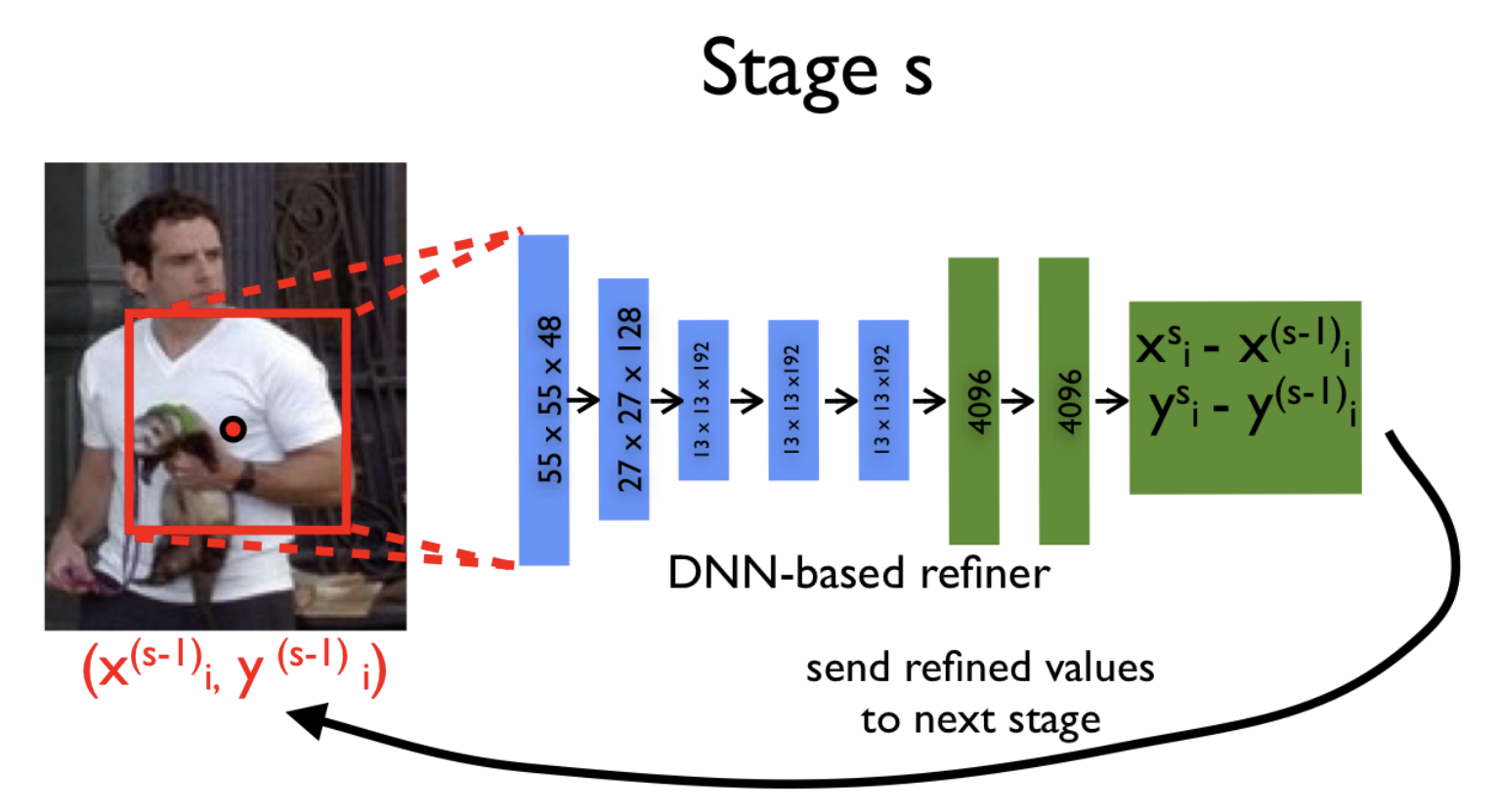
Compromise in the desire to submit to the image in a good resolution and in the need to maintain an adequate number of parameters was the use of a cascade of neural networks. What does it mean? First, from the original image, compressed to pixels, the approximate coordinates of the joints are predicted, and each subsequent neural network specifies these coordinates by a new picture. This new picture is nothing more than some necessary part of the previous one (the same bounding area around the predictions from the previous stage), also reduced to the size .
Thanks to this method, the sequence of models with each step observes images of increasingly higher resolution, which allows the model to focus on fine details and improve the quality of predictions.
Authors use the same network architecture at each stage (total stages ), however, they are taught separately. Let's mark the network parameters at the stage behind and the model itself, predicting the coordinates of the joints, for .
At the initial stage ( ) we use the bounding area (original image completely) to predict the approximate coordinates of the joints:
Further, on each new iteration ( ) and for each joint we specify its coordinates using the model :
And now we could start learning such a model, if it were not for one thing. Training a complex neural network, and even more so a cascade of networks, requires a large number of samples (labeled images, in our case). For example, AlexNet was trained on ImageNet, which consists of 15 million tagged pictures . But even such a dataset Alex and his team increased more than 2048 times, by choosing random smaller subimages and their mirror images.
So that in the considered task the small size of the dataset does not become a serious problem, it was important to come up with a good way to augment data that would be suitable for a cascade of networks.
However, even here the authors found a rather elegant solution. Instead of using the predictions of the coordinates of the joints only from the previous stage, they proposed to generate these coordinates independently. This can be done by shifting the coordinates of a joint to a vector generated from a two-dimensional normal distribution with mean and variance equal to the mean and variance of the observed deviations from for all examples from the training sample.
Thus, we simulate the work of the previous layers on the supposedly new pictures. The cool feature of this method is that we are not limited from above by some fixed number of images that we can generate. However, if there are a lot of them, they will be very similar to each other, and consequently, this will cease to be beneficial.
For the task of estimation, there are two well-known open datasets that researchers often use in their research papers:
The name of this dataset speaks for itself. It represents 5,000 annotated frames from various films. For each picture you need to predict the coordinates of 10 joints.
This dataset consists of photos of people involved in sports. However, not all the photos you get the right idea about him:
But these are rather exceptions, and typical markup examples look like this:
This dataset already contains 12000 images. It differs from FLIC in that it is necessary to predict the coordinates of 14 points instead of 10.
The last thing left for us to understand is to understand how to evaluate the quality of the resulting markup. The authors of the article used two metrics in their work.
This is the percentage of correctly recognized body parts. By part of the body is meant a pair of joints that are interconnected. We believe that we correctly recognized the part of the body, if the distance between the predicted and real coordinates of the two joints does not exceed half of its length. As a result, with the same error, the detection result will depend on the distance between the joints. But despite this flaw, the metric is quite popular.
To compensate for the minuses of the first metric, the authors decided to use another one. Instead of counting the number of correctly recognized parts of the body, it was decided to look at the number of correctly predicted joints. This saves us from depending on the size of the body parts. A joint is considered to be correctly recognized if the distance between the predicted and real coordinates does not exceed a value depending on the size of the body in the picture.
I recall that the above model consists of stages. However, we have not yet clarified how this constant is chosen. In order to find good values for this and other hyperparameters, the article took 50 pictures from both datasets as a validation sample. So the authors stopped at three stages ( ). That is, in the initial image, we get the first approximation of the pose, and then double-refine the coordinates.
Starting from the second stage, 40 images were generated for each joint from a real example. For example, in this way for the LCP dataset (where 14 different joints are predicted), taking into account the mirror images, millions of examples! Another worth noting is that for FLIC as the source bounding box restrictive rectangles obtained by a human-detecting algorithm were used. This allowed pre-cut unnecessary parts of the image.
The first neural network in the cascade was trained on approximately 100 machines for 3 days. However, it is argued that an accuracy close enough to the maximum was achieved in the first 12 hours. At the next stages, each of the models was already trained for 7 days, since it worked with a dataset that was 40 times larger than the original one.
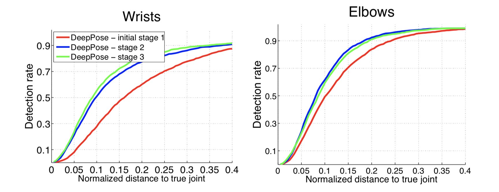
Further on the graphs you can see the recognition accuracy of brushes and elbows at different stages of the model. Along the axis - the value of treshchold in the PDJ metric (if the difference between the predicted and real coordinates is less than treshchold, we believe that the joint is defined correctly). From the graphs it is clear that the additional steps provide a significant improvement in accuracy.
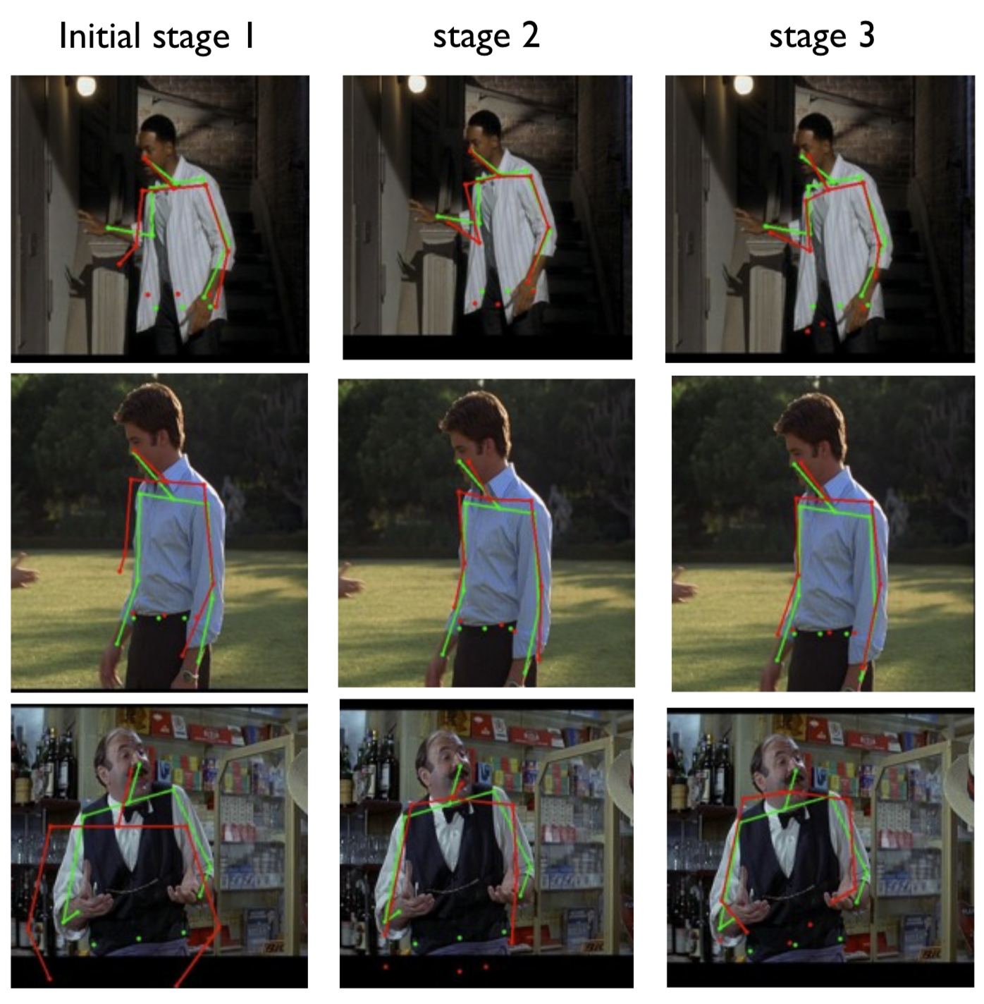
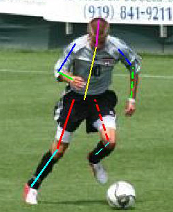
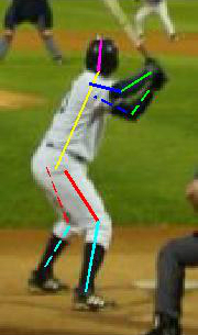
It is also interesting to see how each subsequent neural network specifies the coordinates. On the images below, the true posture is drawn in green and the posture predicted by the model is red.
I will also compare the results of this model with the other five state-of-the-art algorithms of the time.

In my opinion, from the interesting in this work, we can distinguish a method of constructing a model, where by successively connecting several neural networks of the same architecture, it was possible to increase the accuracy quite well. As well as the method of generating additional examples in order to expand the training dataset. I think that thinking about the second is always when you work with a limited set of data. And the more ways you know augmentation, the easier it will come to the right for you.
Post written in collaboration with avgaydashenko .
Today I will tell you about one of the methods for solving the pose estimation problem. The task is to detect body parts in photos, and the method is called DeepPose . This algorithm was proposed by the guys from Google back in 2014. It would seem, not so long ago, but not for the field of deep learning. Since then, many new and more advanced solutions have appeared, but for a full understanding it is necessary to get acquainted with the origins.
Task Overview
Let's first briefly about the formulation of the problem. You have photos in which a person is present (one or more), and you want to mark out body parts on these photos. That is, to say where the hands, legs, head, and so on.
')
Where would such a markup be useful? The first thing that comes to mind is video games. You can play your favorite RPG, swinging a virtual sword, rather than clicking the mouse. To do this, it is enough to be able only to recognize the movements of your hands.
Of course, there are much more practical applications. For example, tracking how customers in a store put goods in their cart, and sometimes put them back on the shelf. Then you can automatically track what the visitor bought, and the need for cash registers will disappear. Amazon has already implemented this idea in its AmazonGo stores.
I think the above examples of use are already interesting enough to take on the task. However, if you have original ideas of where else you can apply the concepts discussed, feel free to write them in the comments.
Classic review
How to solve this problem without neural networks? You can imagine a human skeleton in the form of a graph, where the vertices will be the joints, and the ribs will be the bones. And then come up with some mathematical model that will describe the likelihood of a joint in a particular location of the image, and will also take into account how realistic these joints are located relative to each other. For example, so that your left heel is not on your right shoulder. Although, I do not exclude that there are people capable of it.
One of the options such a mat. The model was implemented in the pictorial structures model framework as early as 1973.
But you can approach the solution of the problem in a less cunning way. When we are given a new picture, let's just search in our original set of tagged pictures that are similar and display its markup. If we initially have not very many different postures of people, then this method is unlikely to take off, but, you see, it is not difficult to implement it. To search for similar images there are usually used classical methods for extracting features from the image processing area: HOG , Fourier descriptor , SIFT, and others.
There are other classic approaches, but here I will not dwell on them and move on to the main part of the post.
New approach
General idea
As you might have guessed, the authors of the article DeepPose (Alexander Toshev, Christian Szegedy) offered their solution using deep neural networks. They decided to consider this problem as a regression problem. That is, for each joint in the photo you need to determine its coordinates.
Data preprocessing
Next, I will continue the description of the model in a more formal language. But for this you need to enter some notation. For convenience, I will stick to the notations of the authors.
Denote the input image as and vector poses as where contains coordinates th joint. That is, we are now representing the human skeleton as a graph from vertices. Then the marked-up image will be denoted as where - our training dataset.
Since the pictures can be of different sizes, as well as the people in the photographs can be represented at different scales and be in different parts of the frame, it was decided to use bounding boxes ( AABB ), which would select the desired image area (the entire human body or more detailed if we are interested in a specific part of the body). Regarding the center of such a region, one can also consider the normalized coordinates of interior points. In the most trivial case, the area can be the entire source image.
Denote the bounding box with the center at wide and tall three numbers .
Then the normalized pose vector regarding the area can be written like this
That is, we subtracted the center of the desired region from all coordinates, and then divided coordinate to the width of the rectangle, and Coordinate height. Now all coordinates began to lie in the interval from before inclusive.
Finally, for denote clipping the original image bounding area . The trivial box, which is equal to the original picture, we denote by .
If we now take the function ( - input image - model parameters, - the number of defined joints), which gives the normalized pose vector, then the pose vector in the original coordinates .
As a function we have a neural network whose weights are described . That is, we feed a three-channel image of a fixed size to the input, and at the output we get joint coordinate pairs:
It would seem that already at this stage we can take some deep neural network (for example, AlexNet, which performed well on the task of image classification, winning the ImageNet competition in 2012) and train it in regression. We will find such model parameters to minimize the sum of squares of deviations of the predicted coordinates from the true ones. That is the ideal parameters . Thus, we are trying to restore the original coordinates of the joints independently of each other.
Cascade of networks
However, since the input to the neural network takes a picture of a fixed size (namely, pixels), some of the information is lost if the picture was originally in the best resolution. Therefore, the model is not possible to analyze all the fine details of the image. The model “sees” everything on a large scale and can try to restore the position only approximately.
It would be possible to simply increase the size of the input, but at the same time, we would have to increase the already large number of parameters inside the grid. Let me remind you that the classic architecture of AlexNet contains more than 60 million parameters! The version of the model described in this article is more than 40 million.
Compromise in the desire to submit to the image in a good resolution and in the need to maintain an adequate number of parameters was the use of a cascade of neural networks. What does it mean? First, from the original image, compressed to pixels, the approximate coordinates of the joints are predicted, and each subsequent neural network specifies these coordinates by a new picture. This new picture is nothing more than some necessary part of the previous one (the same bounding area around the predictions from the previous stage), also reduced to the size .
Thanks to this method, the sequence of models with each step observes images of increasingly higher resolution, which allows the model to focus on fine details and improve the quality of predictions.
Authors use the same network architecture at each stage (total stages ), however, they are taught separately. Let's mark the network parameters at the stage behind and the model itself, predicting the coordinates of the joints, for .
At the initial stage ( ) we use the bounding area (original image completely) to predict the approximate coordinates of the joints:
Further, on each new iteration ( ) and for each joint we specify its coordinates using the model :
Data generation
And now we could start learning such a model, if it were not for one thing. Training a complex neural network, and even more so a cascade of networks, requires a large number of samples (labeled images, in our case). For example, AlexNet was trained on ImageNet, which consists of 15 million tagged pictures . But even such a dataset Alex and his team increased more than 2048 times, by choosing random smaller subimages and their mirror images.
So that in the considered task the small size of the dataset does not become a serious problem, it was important to come up with a good way to augment data that would be suitable for a cascade of networks.
However, even here the authors found a rather elegant solution. Instead of using the predictions of the coordinates of the joints only from the previous stage, they proposed to generate these coordinates independently. This can be done by shifting the coordinates of a joint to a vector generated from a two-dimensional normal distribution with mean and variance equal to the mean and variance of the observed deviations from for all examples from the training sample.
Thus, we simulate the work of the previous layers on the supposedly new pictures. The cool feature of this method is that we are not limited from above by some fixed number of images that we can generate. However, if there are a lot of them, they will be very similar to each other, and consequently, this will cease to be beneficial.
Datasets
For the task of estimation, there are two well-known open datasets that researchers often use in their research papers:
Frames Labeled In Cinema (FLIC)
The name of this dataset speaks for itself. It represents 5,000 annotated frames from various films. For each picture you need to predict the coordinates of 10 joints.
Leeds Sports Pose Dataset (LSP)
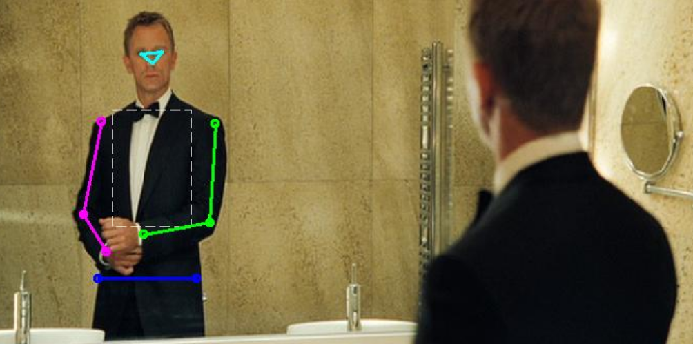
This dataset consists of photos of people involved in sports. However, not all the photos you get the right idea about him:
 |  |
But these are rather exceptions, and typical markup examples look like this:
 |  |  |
This dataset already contains 12000 images. It differs from FLIC in that it is necessary to predict the coordinates of 14 points instead of 10.
Metrics
The last thing left for us to understand is to understand how to evaluate the quality of the resulting markup. The authors of the article used two metrics in their work.
Percentage of Correct Parts (PCP)
This is the percentage of correctly recognized body parts. By part of the body is meant a pair of joints that are interconnected. We believe that we correctly recognized the part of the body, if the distance between the predicted and real coordinates of the two joints does not exceed half of its length. As a result, with the same error, the detection result will depend on the distance between the joints. But despite this flaw, the metric is quite popular.
Percent of Detected Joints (PDJ)
To compensate for the minuses of the first metric, the authors decided to use another one. Instead of counting the number of correctly recognized parts of the body, it was decided to look at the number of correctly predicted joints. This saves us from depending on the size of the body parts. A joint is considered to be correctly recognized if the distance between the predicted and real coordinates does not exceed a value depending on the size of the body in the picture.
Experiment
I recall that the above model consists of stages. However, we have not yet clarified how this constant is chosen. In order to find good values for this and other hyperparameters, the article took 50 pictures from both datasets as a validation sample. So the authors stopped at three stages ( ). That is, in the initial image, we get the first approximation of the pose, and then double-refine the coordinates.
Starting from the second stage, 40 images were generated for each joint from a real example. For example, in this way for the LCP dataset (where 14 different joints are predicted), taking into account the mirror images, millions of examples! Another worth noting is that for FLIC as the source bounding box restrictive rectangles obtained by a human-detecting algorithm were used. This allowed pre-cut unnecessary parts of the image.
The first neural network in the cascade was trained on approximately 100 machines for 3 days. However, it is argued that an accuracy close enough to the maximum was achieved in the first 12 hours. At the next stages, each of the models was already trained for 7 days, since it worked with a dataset that was 40 times larger than the original one.
results
Further on the graphs you can see the recognition accuracy of brushes and elbows at different stages of the model. Along the axis - the value of treshchold in the PDJ metric (if the difference between the predicted and real coordinates is less than treshchold, we believe that the joint is defined correctly). From the graphs it is clear that the additional steps provide a significant improvement in accuracy.
It is also interesting to see how each subsequent neural network specifies the coordinates. On the images below, the true posture is drawn in green and the posture predicted by the model is red.
I will also compare the results of this model with the other five state-of-the-art algorithms of the time.
findings
In my opinion, from the interesting in this work, we can distinguish a method of constructing a model, where by successively connecting several neural networks of the same architecture, it was possible to increase the accuracy quite well. As well as the method of generating additional examples in order to expand the training dataset. I think that thinking about the second is always when you work with a limited set of data. And the more ways you know augmentation, the easier it will come to the right for you.
Post written in collaboration with avgaydashenko .
Source: https://habr.com/ru/post/354850/
All Articles