Apply Gradient Descent on the Real Earth
The usual analogy for explaining gradient descent is this: a person is stuck in the mountains during a heavy fog and must go down. The most logical way is to inspect the surface around and slowly make a path, following down the slope.
This is the essence of the gradient descent, but the analogy is always falling apart when we turn into multidimensional space, the actual geometry of which is little known to us. Although this usually does not become a problem, because gradient descent seems to work quite normally.
But here is an important question: how well is a gradient descent performed on a real Earth?
In the general model, gradient descent selects weights for a model that minimizes the cost function. This is usually some representation of the mistakes made by the model for a number of predictions. But here we do not predict anything, therefore, we do not have “mistakes”, therefore adapting to the journey on the earth requires a little broader context of ordinary machine learning.
')
In our Earth Travel Algorithm, the goal is to reach sea level from any starting position. That is, we will define “weights” as latitude and longitude, and “cost function” as the current altitude above sea level. In other words, the gradient descent should optimize the values of latitude and longitude in such a way as to minimize the height above sea level. Unfortunately, we do not have a mathematical function for the entire earth's surface, therefore, we will calculate the value of the cost based on the raster dataset by altitude from NASA:
Gradient descent takes into account the gradient of the cost function with respect to each variable for which optimization is performed. It adjusts variables to reduce the cost function. This is easy if your cost function is a mathematical metric such as a mean square error. But as we already mentioned, our “cost function” is a search in the database, so there’s nothing to derive from the derivative.
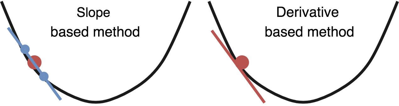
Fortunately, you can approximate a gradient just like the traveler in our analogy: looking around. The gradient is equivalent to the slope, so we estimate the slope by taking a point a little above the current location and a point a little below it (in each dimension) - and divide them to get an estimated derivative. This option should work quite well:
Fine! Notice that this function differs from most implementations of gradient descent in that X or Y variables are not passed to it. Our cost function does not require the calculation of any prediction error, therefore we need only variables that we optimize here. Let's run it on Mount Olympus in Washington:
Hmmm, it looks like he's stuck! The same thing happens when testing in most other places. It turns out that our Earth is crowded with local minima, and the gradient descent is experiencing great difficulties in finding a global minimum if it runs from a local area even near the ocean.
Standard gradient descent is not the only tool, so we will try optimization with inertia (momentum optimization). Inertia is based on real physics, so its application to gradient descent on real geometry is an attractive idea. Unfortunately, if you place even a very large boulder on top of Olympus, it is unlikely that he will have enough inertia to reach the ocean, so you have to use here some unrealistic (in the physical sense) gamma values:
After some adjustment of the variables at the gradient descent, the chances to find the ocean should increase:
Success! It is interesting to observe the behavior of the optimizer. It seems that he fell into the valley and “rolled” from one side to another during the descent, which is consistent with our intuition, as an object with extremely high inertia should behave in the real world.
In reality, the Earth should be a very easy function to optimize. Since it is mostly covered by oceans, more than two thirds of the possible input values for this function return the optimal value of the cost function. But our planet suffers from local minima and nonconvex geography.
I think because of this, it provides many interesting opportunities to study how machine learning optimization methods work on tangible and understandable local geometries. It seems that they did quite well on Olympus, so we’ll assume that the usual analogy for explaining the gradient descent is “confirmed”!
If you have any thoughts on this, let me know on Twitter !
The project code is here .
This is the essence of the gradient descent, but the analogy is always falling apart when we turn into multidimensional space, the actual geometry of which is little known to us. Although this usually does not become a problem, because gradient descent seems to work quite normally.
But here is an important question: how well is a gradient descent performed on a real Earth?
Determination of weights and cost functions
In the general model, gradient descent selects weights for a model that minimizes the cost function. This is usually some representation of the mistakes made by the model for a number of predictions. But here we do not predict anything, therefore, we do not have “mistakes”, therefore adapting to the journey on the earth requires a little broader context of ordinary machine learning.
')
In our Earth Travel Algorithm, the goal is to reach sea level from any starting position. That is, we will define “weights” as latitude and longitude, and “cost function” as the current altitude above sea level. In other words, the gradient descent should optimize the values of latitude and longitude in such a way as to minimize the height above sea level. Unfortunately, we do not have a mathematical function for the entire earth's surface, therefore, we will calculate the value of the cost based on the raster dataset by altitude from NASA:
import rasterio # Open the elevation dataset src = rasterio.open(sys.argv[1]) band = src.read(1) # Fetch the elevation def get_elevation(lat, lon): vals = src.index(lon, lat) return band[vals] # Calculate our 'cost function' def compute_cost(theta): lat, lon = theta[0], theta[1] J = get_elevation(lat, lon) return J Gradient descent takes into account the gradient of the cost function with respect to each variable for which optimization is performed. It adjusts variables to reduce the cost function. This is easy if your cost function is a mathematical metric such as a mean square error. But as we already mentioned, our “cost function” is a search in the database, so there’s nothing to derive from the derivative.
Fortunately, you can approximate a gradient just like the traveler in our analogy: looking around. The gradient is equivalent to the slope, so we estimate the slope by taking a point a little above the current location and a point a little below it (in each dimension) - and divide them to get an estimated derivative. This option should work quite well:
def gradient_descent(theta, alpha, gamma, num_iters): J_history = np.zeros(shape=(num_iters, 3)) velocity = [ 0, 0 ] for i in range(num_iters): cost = compute_cost(theta) # Fetch elevations at offsets in each dimension elev1 = get_elevation(theta[0] + 0.001, theta[1]) elev2 = get_elevation(theta[0] - 0.001, theta[1]) elev3 = get_elevation(theta[0], theta[1] + 0.001) elev4 = get_elevation(theta[0], theta[1] - 0.001) J_history[i] = [ cost, theta[0], theta[1] ] if cost <= 0: return theta, J_history # Calculate slope lat_slope = elev1 / elev2 - 1 lon_slope = elev3 / elev4 - 1 # Update variables theta[0][0] = theta[0][0] - lat_slope theta[1][0] = theta[1][0] - lon_slope return theta, J_history Fine! Notice that this function differs from most implementations of gradient descent in that X or Y variables are not passed to it. Our cost function does not require the calculation of any prediction error, therefore we need only variables that we optimize here. Let's run it on Mount Olympus in Washington:
Hmmm, it looks like he's stuck! The same thing happens when testing in most other places. It turns out that our Earth is crowded with local minima, and the gradient descent is experiencing great difficulties in finding a global minimum if it runs from a local area even near the ocean.
Optimization with inertia
Standard gradient descent is not the only tool, so we will try optimization with inertia (momentum optimization). Inertia is based on real physics, so its application to gradient descent on real geometry is an attractive idea. Unfortunately, if you place even a very large boulder on top of Olympus, it is unlikely that he will have enough inertia to reach the ocean, so you have to use here some unrealistic (in the physical sense) gamma values:
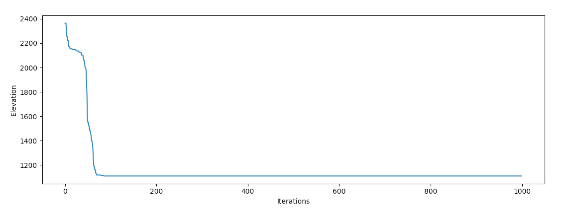
def gradient_descent(theta, alpha, gamma, num_iters): J_history = np.zeros(shape=(num_iters, 3)) velocity = [ 0, 0 ] for i in range(num_iters): cost = compute_cost(theta) # Fetch elevations at offsets in each dimension elev1 = get_elevation(theta[0] + 0.001, theta[1]) elev2 = get_elevation(theta[0] - 0.001, theta[1]) elev3 = get_elevation(theta[0], theta[1] + 0.001) elev4 = get_elevation(theta[0], theta[1] - 0.001) J_history[i] = [ cost, theta[0], theta[1] ] if cost <= 0: return theta, J_history # Calculate slope lat_slope = elev1 / elev2 - 1 lon_slope = elev3 / elev4 - 1 # Calculate update with momentum velocity[0] = gamma * velocity[0] + alpha * lat_slope velocity[1] = gamma * velocity[1] + alpha * lon_slope # Update variables theta[0][0] = theta[0][0] - velocity[0] theta[1][0] = theta[1][0] - velocity[1] return theta, J_history After some adjustment of the variables at the gradient descent, the chances to find the ocean should increase:
Success! It is interesting to observe the behavior of the optimizer. It seems that he fell into the valley and “rolled” from one side to another during the descent, which is consistent with our intuition, as an object with extremely high inertia should behave in the real world.
Final thoughts
In reality, the Earth should be a very easy function to optimize. Since it is mostly covered by oceans, more than two thirds of the possible input values for this function return the optimal value of the cost function. But our planet suffers from local minima and nonconvex geography.
I think because of this, it provides many interesting opportunities to study how machine learning optimization methods work on tangible and understandable local geometries. It seems that they did quite well on Olympus, so we’ll assume that the usual analogy for explaining the gradient descent is “confirmed”!
If you have any thoughts on this, let me know on Twitter !
The project code is here .
Source: https://habr.com/ru/post/354772/
All Articles