Developing a simple deep learning model for predicting stock prices using TensorFlow

Data science expert and STATWORX CEO Sebastian Heinz published on Medium a guide to creating a deep learning model for predicting stock prices on a stock exchange using the TensorFlow framework. We have prepared an adapted version of this useful material.

The author posted the final Python script and compressed dataset in his repository on GitHub .
')

Import and prepare data

Heinz exported stock data to a csv file. His dataset contained n = 41266 minutes of data, covering 500 trades in shares from April to August 2017, and also included information on the price of the S & P 500 index.

#   data = pd.read_csv('data_stocks.csv') #   date data = data.drop(['DATE'], 1) #   n = data.shape[0] p = data.shape[1] #    numpy- data = data.values

This is the S & P index time series, built using pyplot.plot (data ['SP500']):

An interesting point: since the ultimate goal is to “predict” the index value in the near future, its value shifts one minute ahead.

Preparation of data for testing and training

The data set was divided into two - one part for testing, and the second for training. At the same time, data for training accounted for 80% of their total volume and covered the period from April to approximately the end of July 2017, the data for testing ended in August 2017.

 #      train_start = 0 train_end = int(np.floor(0.8*n)) test_start = train_end test_end = n data_train = data[np.arange(train_start, train_end), :] data_test = data[np.arange(test_start, test_end), :]

There are many approaches to cross-validation of time series, from generating forecasts with or without reconfiguration of the model (refitting) to more complex concepts like bootstrap-resampling of time series. In the latter case, the data is broken up into repeated samples from the beginning of the seasonal time series decomposition — this allows you to simulate samples that follow the same seasonal pattern as the original time series, but do not completely copy its values.

Data scaling

Most neural network architectures use input scaling (and sometimes output). The reason is that most neuron activation functions like sigmoid or hyperbolic tangent ( tanx ) are defined at intervals [-1, 1] or [0, 1], respectively. Currently, the most commonly used activation of the rectified linear unit (ReLU). Heinz decided to scale the input data and goals using MinMaxScaler in Python for this purpose:

 #   from sklearn.preprocessing import MinMaxScaler scaler = MinMaxScaler() scaler.fit(data_train) data_train = scaler.transform(data_train) data_test = scaler.transform(data_test) #  X  y X_train = data_train[:, 1:] y_train = data_train[:, 0] X_test = data_test[:, 1:] y_test = data_test[:, 0]

Note : Care should be taken when selecting a piece of data and time for scaling. A common mistake here is to scale the entire dataset before splitting it into test and training data. This is an error, because scaling starts counting statistics, that is, the minima / maxima of variables. When realizing time series forecasting in real life, at the time of their generation you cannot have information from future observations. Therefore, statistics should be calculated on training data, and then the result obtained should be applied to test data. Taking information “from the future” (that is, from a test sample) to generate predictions, the model will issue predictions with a “system bias” (bias).

Introduction to TensorFlow

TensorFlow is an excellent product, currently it is the most popular framework for solving machine learning problems and creating neural networks. The product backend is based on C ++, but Python is usually used for management (there is also a wonderful TensorFlow library for R ). TensorFlow uses the concept of graphical representation of computational problems. This approach allows users to define mathematical operations as data graph elements, variables, and operators. Since neural networks, in fact, are graphs of data and mathematical operations, TensorFlow is great for working with them and machine learning. In the example below, a graph is presented that solves the problem of adding two numbers:

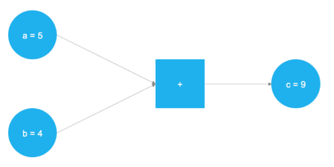
The figure above shows two numbers that need to be folded. They are stored in variables a and b. The values travel along the graph and fall into a node represented by a square, where addition occurs. The result of the operation is written to another variable c. Used variables can be considered as placeholders. Any numbers that fall into a and b are added together, and the result is written in c.

This is exactly how TensorFlow works - the user defines an abstract representation of a model (neural network) through placeholders and variables. After that, the first ones are filled with real data and calculations take place. The test example above is described by the following code in TensorFlow:

 #  TensorFlow import tensorflow as tf #  a  b    a = tf.placeholder(dtype=tf.int8) b = tf.placeholder(dtype=tf.int8) #   c = tf.add(a, b) #   graph = tf.Session() #   graph.run(c, feed_dict={a: 5, b: 4})

After importing the TensorFlow library using tf.placeholder (), two placeholders are defined. They correspond to the two blue circles on the left side of the image above. After that, using tf.add () is determined by the operation of addition. The result of the operation is c = 9. With tuned placeholders, the graph can be executed for any integer values a and b. It is clear that this example is extremely simple, and neural networks in real life is much more complicated, but it allows you to understand the principles of the framework.

Placeholders

As stated above, everything starts with placeholders. In order to implement a model, you need two such elements: X contains input data for the network (stock prices of all S & P 500 elements at time T = t) and output data Y (S & P 500 index values at time T = t + 1) .

The form of placeholders corresponds to [None, n_stocks], where [None] means that the input data is represented as a two-dimensional matrix, and the output data is a one-dimensional vector. It is important to understand what form of input and output data neural networks need and organize them accordingly.

 #  X = tf.placeholder(dtype=tf.float32, shape=[None, n_stocks]) Y = tf.placeholder(dtype=tf.float32, shape=[None])

Argument None means that at this point we do not yet know the number of observations that will pass through the graph of the neural network during each launch, so it remains flexible. Later, the variable batch_size, which controls the number of observations during the training run, will be defined.

Variables

In addition to placeholders, there is another important element in the TensorFlow universe - these are variables. If placeholders are used to store input and target data in a graph, then the variables serve as flexible containers inside the graph. They are allowed to change during the execution of the graph. Weights and offsets are represented by variables in order to facilitate adaptation during training. Variables must be initialized before learning.

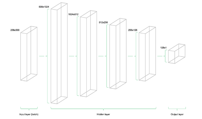
The model consists of four hidden levels. The first contains 1024 neurons, which is a little more than twice the amount of input data. Subsequent hidden levels are always two times less than the previous one - they combine 512, 256 and 128 neurons. The reduction in the number of neurons at each level compresses the information that the network has processed at the previous levels. There are other neuron architectures and configurations, but this tutorial uses exactly this model:

 #    n_stocks = 500 n_neurons_1 = 1024 n_neurons_2 = 512 n_neurons_3 = 256 n_neurons_4 = 128 n_target = 1 #  1:       W_hidden_1 = tf.Variable(weight_initializer([n_stocks, n_neurons_1])) bias_hidden_1 = tf.Variable(bias_initializer([n_neurons_1])) #  2:       W_hidden_2 = tf.Variable(weight_initializer([n_neurons_1, n_neurons_2])) bias_hidden_2 = tf.Variable(bias_initializer([n_neurons_2])) #  3:       W_hidden_3 = tf.Variable(weight_initializer([n_neurons_2, n_neurons_3])) bias_hidden_3 = tf.Variable(bias_initializer([n_neurons_3])) #  4:       W_hidden_4 = tf.Variable(weight_initializer([n_neurons_3, n_neurons_4])) bias_hidden_4 = tf.Variable(bias_initializer([n_neurons_4])) #   :       W_out = tf.Variable(weight_initializer([n_neurons_4, n_target])) bias_out = tf.Variable(bias_initializer([n_target]))

It is important to understand what variable sizes are required for different levels. The rule of thumb of multi-level perceptrons is that the size of the previous level is the first size of the current level for weights matrices. It sounds difficult, but the point is that each level transmits its output as input to the next level. The sizes of the displacements are equal to the second size of the weights matrix of the current level, which corresponds to the number of neurons in the level.

Network architecture design

After determining the required weights and offsets of the variables, the network topology, it is necessary to determine the network architecture. Thus, placeholders (data) and variables (weights and displacements) need to be combined into a system of successive matrix multiplications. Hidden network levels are transformed by activation functions. These functions are important elements of the network infrastructure, since they introduce nonlinearity into the system. There are dozens of activation functions, and one of the most common is rectified linear unit (ReLU). It is this manual that is used in this manual:

 #   hidden_1 = tf.nn.relu(tf.add(tf.matmul(X, W_hidden_1), bias_hidden_1)) hidden_2 = tf.nn.relu(tf.add(tf.matmul(hidden_1, W_hidden_2), bias_hidden_2)) hidden_3 = tf.nn.relu(tf.add(tf.matmul(hidden_2, W_hidden_3), bias_hidden_3)) hidden_4 = tf.nn.relu(tf.add(tf.matmul(hidden_3, W_hidden_4), bias_hidden_4)) #   (  ) out = tf.transpose(tf.add(tf.matmul(hidden_4, W_out), bias_out))

The image below illustrates the network architecture. The model consists of three main blocks. The level of input data, hidden levels and output level. This infrastructure is called a feedforward network. This means that chunks of data move along the structure strictly from left to right. In other implementations, for example, in the case of recurrent neural networks, data can flow inside the network in different directions.

Cost function

The network cost function is used to generate an estimate of the variance between network predictions and actual observation results during training. To solve regression problems, use the mean square error function (MSE). This function calculates the standard deviation between predictions and goals, but in general, any differentiated function can be used to calculate the deviation between the two.

 #   mse = tf.reduce_mean(tf.squared_difference(out, Y))

In doing so, MSE displays specific entities that are useful for solving a general optimization problem.

Optimizer

The optimizer undertakes the necessary calculations required to adapt the weights and variable deviations of the neural network during training. These calculations lead to calculations of the so-called gradients, which indicate the direction of the necessary change in the deviations and weights to minimize the cost function. Developing a stable and fast optimizer is one of the main tasks of the creators of neural networks.

 #  opt = tf.train.AdamOptimizer().minimize(mse)

In this case, use one of the most common optimizers in the field of machine learning Adam Optimizer. Adam is an abbreviation for the phrase “Adaptive Moment Estimation” (adaptive estimation of moments), it is a cross between two other popular optimizers AdaGrad and RMSProp

Initializers

Initializers are used to initialize variables before starting learning. Since neural networks are trained using numerical optimization techniques, the starting points of an optimization problem are one of the most important factors in the search for a good solution. There are different initializers in TensorFlow, each of which uses its own approach. This tutorial uses tf.variance_scaling_initializer (), which implements one of the standard initialization strategies.

 #  sigma = 1 weight_initializer = tf.variance_scaling_initializer(mode="fan_avg", distribution="uniform", scale=sigma) bias_initializer = tf.zeros_initializer()

Note: In TensorFlow, you can define several initialization functions for different variables within a graph. However, in most cases, a fairly unified initialization.

Neural network setup

After determining the placeholders, variables, initializers, cost functions, and optimizers, the model must be trained. Usually this is done using the mini-batches training approach. In the course of such training, random samples of size n = batch_size are selected from the data set for training and loaded into the neural network. The training dataset is divided into n / batch_size pieces, which are then sequentially sent to the network. At this point, the placeholders X and Y come into play. They store the input and target data and send them to the neural network.

The sampled X data passes through the network to reach the output level. Then TensorFlow compares the model-generated predictions with the actually observed goals Y in the current “run”. After that, TensorFlow performs the optimization step and updates the network parameters. After the weights and deviations are updated, the process is repeated again for a new piece of data. The procedure is repeated until all the “sliced” pieces of data are sent to the neural network. The full cycle of such processing is called the "epoch".

Network training stops when the maximum number of epochs is reached or when another predetermined stopping criterion is triggered.

 #   net = tf.Session() #   net.run(tf.global_variables_initializer()) #    plt.ion() fig = plt.figure() ax1 = fig.add_subplot(111) line1, = ax1.plot(y_test) line2, = ax1.plot(y_test*0.5) plt.show() #       epochs = 10 batch_size = 256 for e in range(epochs): #     shuffle_indices = np.random.permutation(np.arange(len(y_train))) X_train = X_train[shuffle_indices] y_train = y_train[shuffle_indices] #  - for i in range(0, len(y_train) // batch_size): start = i * batch_size batch_x = X_train[start:start + batch_size] batch_y = y_train[start:start + batch_size] # Run optimizer with batch net.run(opt, feed_dict={X: batch_x, Y: batch_y}) #   if np.mod(i, 5) == 0: # Prediction pred = net.run(out, feed_dict={X: X_test}) line2.set_ydata(pred) plt.title('Epoch ' + str(e) + ', Batch ' + str(i)) file_name = 'img/epoch_' + str(e) + '_batch_' + str(i) + '.jpg' plt.savefig(file_name) plt.pause(0.01) #    MSE   mse_final = net.run(mse, feed_dict={X: X_test, Y: y_test}) print(mse_final)

During the training, the predictions generated by the network on the test set were evaluated, then visualization was performed. In addition, the images were uploaded to the disk and later, video-animation of the learning process was created from them:

As you can see, the neural network quickly adapts to the basic form of the time series and continues to search for the best data patterns. After 10 epochs, we get results very close to the test data. The final value of the MSE function is 0.00078 (a very small value due to the fact that the goals are scaled). The average absolute percentage error of the forecast on the test set is 5.31% - a very good result. It is important to understand that this is only a coincidence with test data, and not real data.

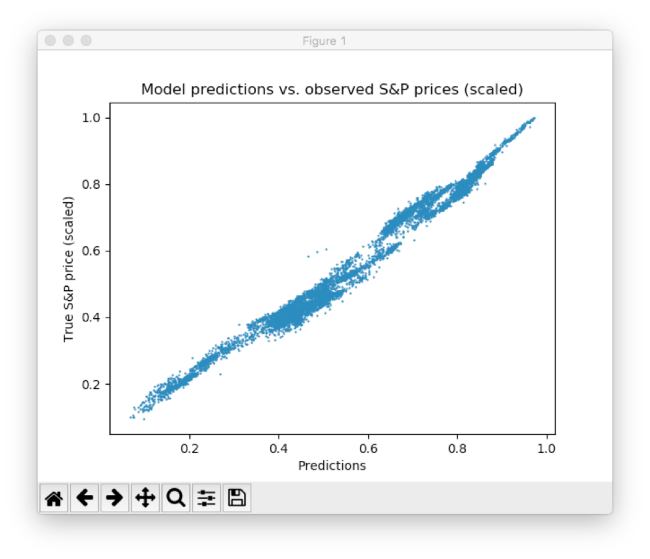
Scatter plot between predicted and real S & P prices

This result can be further improved in many ways, from the elaboration of levels and neurons, to the choice of other initialization and activation schemes. In addition, various types of deep learning models can be used, such as recurrent neural networks - this can also lead to better results.

Other materials on finance and stock market from ITI Capital :

Source: https://habr.com/ru/post/354732/

All Articles