The solution to the problem of detecting the center line of the vessel

The essence of the task

In the process of medical diagnosis, it may be necessary to examine the vessels of the patient. Such a study is called angiography. With the advent of tomographs, in addition to classical angiography, MRI and CT angiography methods have appeared, which, in contrast to traditional angiography, which gives only a flat image in one projection, allows us to obtain a complete three-dimensional representation of the vessels. To carry out such studies, a contrast is injected into the patient’s blood — a special substance that makes the vessels in the pictures brighter. Depending on the intended diagnosis, the doctor either assesses the overall picture, or tries to find specific areas of the vessels in which problems have arisen. If a portion of the vessel is narrowed and transmits less blood than it should, then this place is called stenosis.


One of the tasks of a doctor is to find stenoses and assess how dangerous they are. The task of the developer, as usual, to facilitate the work of the end user. To do this, it is necessary to build a full 3D model of the vessel walls and conduct their primary analysis. This is a big and interesting task, however, it is based on a more simple and well-known problem - the construction of the central line of the vessel.

First try

Before continuing to read this article, it is advisable to get a little familiar with the presentation of the data obtained from the work of tomographs. This can be done by reading our long-written article about the voxel render of the DICOM Viewer from the inside . In short: there is a 3D array of numbers, in each element of which the signal value (intensity) is stored. This array is called volume. The element itself is a voxel, and its indices in the 3D array will be 3D coordinates. Before the rendering of each voxel, its intensity is processed by the function, and the voxel acquires a certain color, brightness and transparency.

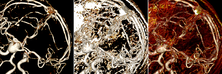
Regarding the task, the first thing I encountered was that our render allows us to show all the vessels at the visual level. Namely, from an incomprehensible “porridge”, as in the figure on the left, playing around with the settings you can make quite obvious vessels, as in the figure on the right:
')

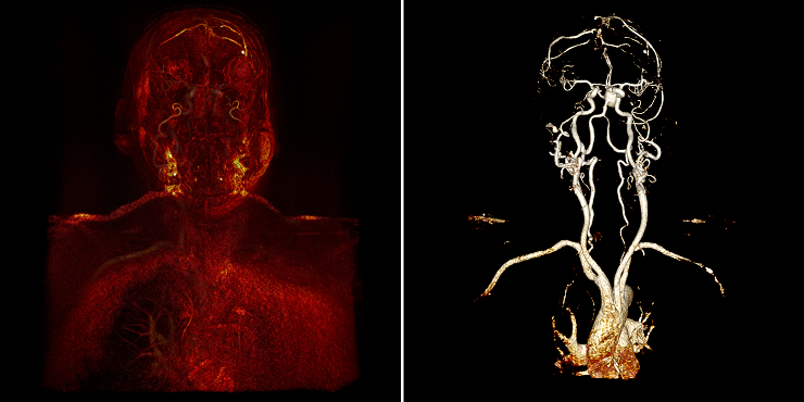
It seems that the problem is solved: “here they are” vessels, a region growing algorithm immediately comes to mind: we know the color and transparency of the voxels we need, which means we can iterate through their neighbors until the path between the specified points has been laid.


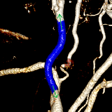
In addition, the idea comes that if you deal with the branches, you can extend the entire network of vessels. But the reality is not so simple. The vessel can fit closely to the bones (their voxels are identical in color, so the bone will be perceived as part of the vessel):


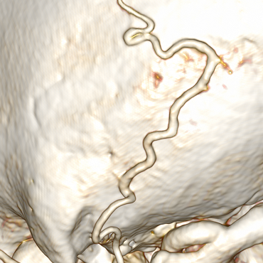
The vessel may curl or fit close to itself:


Parts of the vessel can be very thin and even interrupted:


Finding optimal render settings is nontrivial. The user can change the so-called window, and there is no specific value of the window suitable for all vessels of at least the same study. The window has to be customized each time for a specific case. Below are three options for the same place with different settings:


As a result, we come to the fact that the intuitively seemingly correct algorithm needs to either be refined, or a completely different approach should be tried. After a lot of unsuccessful attempts, I had to try something else.

Classic approach

The main approach to the problem of vessel detection (vessel detection) is to calculate the eigenvalues ​​of the Hessian matrix. Also recently, they are trying to connect neural networks to this task. However, the standard solution looks more reliable because it is mentioned in more literature and is used not only for finding vessels, but also for many other tasks (for example, detecting objects in astronomical images), so neural networks had to be abandoned.

In our case, the Hesse matrix is ​​a matrix whose elements are partial derivatives of the second order of intensity in a particular voxel:

$$

$$H_ {M} = \ begin {pmatrix} \ frac {\ partial ^ 2 f} {\ partial ^ 2 x} & \ frac {\ partial ^ 2 f} {\ partial x \ partial y} & \ frac {\ partial ^ 2 f} {\ partial x \ partial z} \\ \ frac {\ partial ^ 2 f} {\ partial x \ partial y} & \ frac {\ partial ^ 2 f} {\ partial ^ 2 y} & \ frac {\ partial ^ 2 f} {\ partial y \ partial z} \\ \ frac {\ partial ^ 2 f} {\ partial x \ partial z} & \ frac {\ partial ^ 2 f} {\ partial y \ partial z} & \ frac {\ partial ^ 2 f} {\ partial ^ 2 z} \ end {pmatrix}$$

- accordingly, the second partial derivatives.

After constructing the Hesse matrix, it is necessary to find its eigenvalues ​​and eigenvectors by solving the following equation:

$$

$$\ begin {vmatrix} \ frac {\ partial ^ 2 f} {\ partial ^ 2 x} - \ lambda_ {1} & \ frac {\ partial ^ 2 f} {\ partial x \ partial y} & \ frac { \ partial ^ 2 f} {\ partial x \ partial z} \\ \ frac {\ partial ^ 2 f} {\ partial x \ partial y} & \ frac {\ partial ^ 2 f} {\ partial ^ 2 y} - \ lambda_ {2} & \ frac {\ partial ^ 2 f} {\ partial y \ partial z} \\ \ frac {\ partial ^ 2 f} {\ partial x \ partial z} & \ frac {\ partial ^ 2 f} {\ partial y \ partial z} & \ frac {\ partial ^ 2 f} {\ partial ^ 2 z} - \ lambda_ {3} \ end {vmatrix} = 0$$

- own values. The problem of finding them is reduced to solving a cubic equation, but in our case the matrix is ​​symmetric, so the solution is simplified and can be represented by a small pseudo-code:

p1 = A(1,2)^2 + A(1,3)^2 + A(2,3)^2 if (p1 == 0) eig1 = A(1,1) eig2 = A(2,2) eig3 = A(3,3) else q = trace(A)/3 p2 = (A(1,1) - q)^2 + (A(2,2) - q)^2 + (A(3,3) - q)^2 + 2 * p1 p = sqrt(p2 / 6) B = (1 / p) * (A - q * I) r = det(B) / 2 if (r <= -1) phi = pi / 3 else if (r >= 1) phi = 0 else phi = acos(r) / 3 end eig1 = q + 2 * p * cos(phi) eig3 = q + 2 * p * cos(phi + (2*pi/3)) eig2 = 3 * q - eig1 - eig3 end 

Where A is the original 3x3 matrix; I - 3x3 identity matrix; eig1, eig2, eig2 - eigenvalues; trace () - returns the trace of the matrix; det () - returns the determinant of the matrix.

Now we can find eigenvectors. To do this in the equation:

$$

$$\ begin {vmatrix} \ frac {\ partial ^ 2 f} {\ partial ^ 2 x} - \ lambda & \ frac {\ partial ^ 2 f} {\ partial x \ partial y} & \ frac {\ partial ^ 2 f} {\ partial x \ partial z} \\ \ frac {\ partial ^ 2 f} {\ partial x \ partial y} & \ frac {\ partial ^ 2 f} {\ partial ^ 2 y} - \ lambda & \ frac {\ partial ^ 2 f} {\ partial y \ partial z} \\ \ frac {\ partial ^ 2 f} {\ partial x \ partial z} & \ frac {\ partial ^ 2 f} {\ partial y \ partial z} & \ frac {\ partial ^ 2 f} {\ partial ^ 2 z} - \ lambda \ end {vmatrix} \ cdot \ begin {vmatrix} V_ {x} \\ V_ {y} \\ V_ {z} \ end {vmatrix} = 0$$

substitute one of the found eigenvalues ​​instead of . Found vector and will be a private vector. There are three such vectors: - one for each eigenvalue. Eigenvalues ​​and vectors must be sorted in this order. while the vectors also change places, i.e. swapping values and we also change places and . If after sorting the condition , it is considered that the voxel in which the matrix was built belongs to the vessel. At the same time own vector will indicate the direction along the vessel no matter how close the voxel is to the wall:


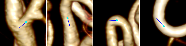
If the voxel belongs to a vessel, the so-called vascularity is calculated on the basis of the eigenvalues ​​of the matrix. There are a lot of different formulas in the literature, and we adapted one of them for ourselves:

$$

$$V _ {\ sigma} = \ left (1- \ frac {{\ lvert} {\ lvert} \ lambda_ {2} {\ rvert} - {\ lvert} \ lambda_ {3} {\ rvert} {\ rvert} } {{\ lvert} \ lambda_ {2} {\ rvert} + {\ lvert} \ lambda_ {3} {\ rvert}} \ right) \ cdot \ left (\ lambda_ {1} \ frac {2} {3 } - \ lambda_ {2} - \ lambda_ {3} \ right) \ cdot \ left (1-e ^ {- \ frac {{\ lambda_ {1}} ^ 2 + {\ lambda_ {2}} ^ 2+ {\ lambda_ {3}} ^ 2} {2}} \ right)$$

- accordingly, the value of vascularity

The more vascular, the closer the voxel to the center of the vessel. Now it is easy to imagine a simple algorithm for finding the center line from a given voxel:

1. Determine the direction of the vessel in the current voxel,
2. Make a cut of the vessel perpendicular to the direction and move along the gradient to the cut voxel with maximum vascularity,
3. Determine the direction of the vessel in the voxel with maximum vascularity,
4. We take a small step in the direction of the vessel and get into the new voxel,
5. Go back to step 1.

From the original point, the movement occurs in two directions, because we cannot know in advance which of them we need:


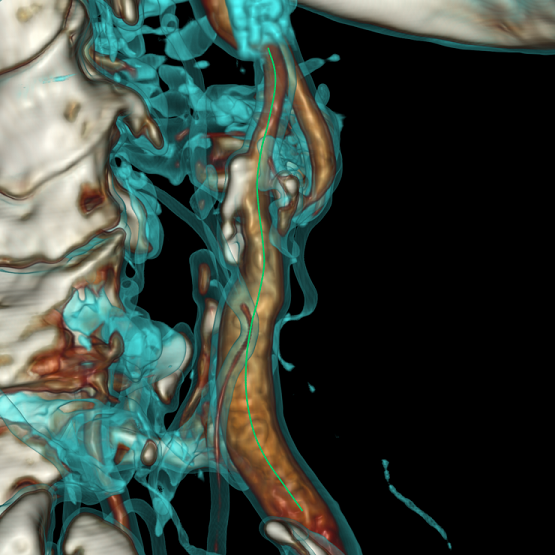
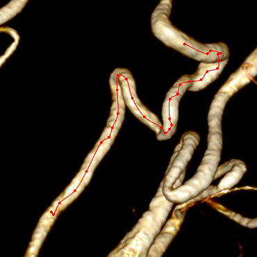
As a result, we get not the most beautiful, but the correct center line:



To make the center line less angular, you need to abandon the integer coordinates of the voxels and move to the fractional coordinates of points in 3D space; you can also perform a slight smoothing of the center line after construction.

To go to the fractional coordinates, we used the bicubic interpolation when obtaining the intensity values. The general equation of the filter in one-dimensional space is as follows:

$$

$$k (x) = \ frac {1} {6} \ begin {cases} (12-9B-6C) \ lvert {x} \ rvert ^ 3 + (- 18 + 12B + 6C) \ lvert {x} \ rvert ^ 2 + (6-2B), \ quad if \> \ lvert {x} \ rvert <1 \\ (- B-6C) \ lvert {x} \ rvert ^ 3 + (6B + 30C) \ lvert { x} \ rvert ^ 2 + (- 12B-48C) \ lvert {x} \ rvert + (8B + 24C), \\ if \> 1 \ leq \ lvert {x} \ rvert <2 \\ 0, \ quad otherwise \ end {cases}$$

Where and have predefined values. If a then we are dealing with b-spline if , then with a cardinal spline. In our case , (Catmull-Rom filter). Then we get:

$$

$$k (x) = \ frac {1} {6} \ begin {cases} 9 \ lvert {x} \ rvert ^ 3-15 \ lvert {x} \ rvert ^ 2 + 6, \ quad if \> \ lvert {x} \ rvert <1 \\ - 3 \ lvert {x} \ rvert ^ 3 + 15 \ lvert {x} \ rvert ^ 2-24 \ lvert {x} \ rvert + 12, \ quad if \> 1 \ leq \ lvert {x} \ rvert <2 \\ 0, \ quad otherwise \ end {cases}$$

Consider the case for 1D. If given values ​​are in points with coordinates and we interpolate where , then we can calculate the weight for each vertex:

$$

$$\\ w _ {- 1} (x) = \ frac {1} {2} (x ^ 2 (2-x) -x) \\ w_ {0} (x) = \ frac {1} {2} (x ^ 2 (3x-5) +2) \\ w_ {1} (x) = \ frac {1} {2} (x ^ 2 (4-3x) + x) \\ w_ {2} (x ) = \ frac {1} {2} x ^ 2 (x-1)$$

Total predicted value:

$$

$$f (x) = p _ {- 1} \ cdot w _ {- 1} (x) + p_ {0} \ cdot w_ {0} (x) + p_ {1} \ cdot w_ {1} (x) + p_ {2} \ cdot w_ {2} (x)$$

Now consider our full case for 3D space. As you might guess, we will interpolate inside the cube with the dimension of 4x4x4 voxel. We take as a basis the weights considered for the 1D case:

$$

$$f (x_ {0}, y_ {0}, z_ {0}) = \ sum_ {i = -1} ^ {2} \ sum_ {j = -1} ^ {2} \ sum_ {k = -1 } ^ {2} w_ {i} (x_ {0} - \ lfloor x_ {0} \ rfloor) \ cdot w_ {j} (y_ {0} - \ lfloor y_ {0} \ rfloor) \ cdot w_ {k } (z_ {0} - \ lfloor z_ {0} \ rfloor) \ cdot \\\ cdot I (\ lfloor x_ {0} \ rfloor + i, \ lfloor y_ {0} \ rfloor + j, \ lfloor z_ { 0} \ rfloor + k)$$

Where - fractional coordinates of a point, - intensity in the voxel with coordinates , - rounding down.

It may seem interesting to someone that the sum of the weights of all voxels is 1:

$$

$$\ sum_ {i = -1} ^ {2} \ sum_ {j = -1} ^ {2} \ sum_ {k = -1} ^ {2} w_ {i} (x- \ lfloor x \ rfloor) \ cdot w_ {j} (y- \ lfloor y \ rfloor) \ cdot w_ {k} (z- \ lfloor z \ rfloor) = 1$$

Details

Let us return to the calculation of derivatives for the Hesse matrix. We have coordinates and intensity, as the second partial derivative is numerically considered as everyone knows: the basic is the finite difference method. For point :


To eliminate noise, before calculating the derivatives, it is necessary to perform a Gaussian smoothing with a certain value. and only then calculate the Hessian matrix at a specific point already on the smoothed intensity values. Gaussian smoothing at :

$$

$$G (x_ {0}, y_ {0}, z_ {0}) = \ sum_ {i = -r} ^ {r} \ sum_ {j = -r} ^ {r} \ sum_ {k = -r } ^ {r} I (x_ {0} + i, y_ {0} + j, z_ {0} + k) \ cdot \ frac {1} {(2 \ pi) ^ \ frac {3} {2} \ sigma ^ 3} \ cdot {e} ^ {- \ frac {i ^ 2 + j ^ 2 + k ^ 2} {2 \ sigma ^ 2}}$$

Where returns the intensity value at the point ; usually takes value ( - rounding up); - smoothing factor.

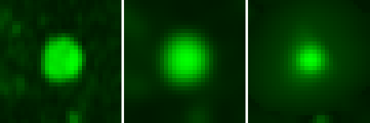
The intensity values ​​in the perpendicular section of the vessel before smoothing, after smoothing, in the third figure, the values ​​of vascularity:


In this case, the greater the value we use, the thicker the vessels we try to find . And since we need all vessels in general - both thin and thick, we need many meanings. , and for each value we need to perform a smoothing. We stopped at the range which includes 10 values.

However, with increasing values ​​of the second derivatives decrease. This, in turn, leads to the fact that vascularity, calculated with a large , it turns out to be less vascular, calculated at the same point with a small , even if in reality we are dealing with a thick vessel. It turns out that, regardless of the real picture, structures resembling thin vessels always prevail. Therefore, the question arises: how to correlate with each other all the obtained vascularity for each of ? To do this, you must perform a normalization between the results of the calculations. In the literature, manipulations with the obtained vascularity are usually carried out, for example:

where - normalized vascularity - vascularity obtained for smoothing with , It is selected experimentally, a good option is 0.5.

We used the so-called gamma normalization: where - Hesse matrix, - order of the derivative, i.e. 2, is chosen experimentally, in our case, version 0.5 showed itself well. Then the whole formula comes down to .

Now, if we try to calculate the value of vascularity with a small in the center of a perfectly thin vessel, it will be approximately equal to the value of vascularity with a large for the center of an ideally thick vessel.

The calculation algorithm for an arbitrary point when building the center line looks like this:

1. • select value and perform smoothing at a point and in its neighbors (they are needed to calculate the derivatives),
   • calculate the second derivatives and build the Hesse matrix,
   • normalize the Hesse matrix by multiplying it by , and find eigenvalues,
     
   • calculate vascularity
   • if there are unused then go back to the beginning, otherwise go to point 2.
2. Calculate the eigenvectors of the Hesse matrix, for which the vascularity turned out to be maximum, and obtain the vector-direction of the vessel.

Combining this algorithm with the algorithm for building the center line, we get the final result:

Optimization

The approach described above will work fine, but there are a few points. First, to improve performance, smoothing must be performed in advance for all voxels and for all . Secondly, given that studies typically have a size of about 512x512x512 voxels, the size of the memory required to store the results of smoothing will on average take about 5 GB. To reduce the amount of memory consumed, we used the pyramid (scale space pyramid).

The idea is that since after each smoothing, the intensity values ​​in the neighboring voxels blur and become approximately equal, there is no point in storing them all. Those. the more , the less we then need calculated voxels to restore smoothing throughout the volume.

In general, it works like this. The zero volume layer is original. A smoothing filter (¼, ½, ¼) is applied several times along each of the volume axes, and after that the dimensionality of the volume is halved. The resulting volume will belong to the first layer. Then the operation is repeated and the second layer is obtained. Then the third, etc. Each layer corresponds to a specific value. . Example for 2D: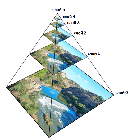

It is easy to calculate that in 3D the total amount of memory will be equal to where - the amount of memory required to store the original volume. However, the use of the pyramid conceals a lot of difficulties and problems that we have encountered, and which pull on a separate article, if you talk about them.

Total

It can be considered that the described approach to building the center line is extremely effective, but it has some drawbacks:

1. For CT studies, it is not possible to detect vessels that pass inside the bones (as, for example, in the spine)
2. It is not always possible to detect vessels if they pass near elongated elongated bones, tissues or structures (in such cases bones, tissues and structures themselves may be mistaken for vessels)
3. The bottleneck is bifurcations (bifurcation of vessels)

Problems 1 and 2 are solved by subtracting the bones. For this, two CT examinations are necessary - with and without contrast. It is clear that the only difference between such studies will be illuminated vessels. In other words, if we subtract the intensity of each voxel of a study without vessels from the intensity of each voxel of a study with vessels, then as a result only vessels related to vessels will have non-zero intensity. But since the two studies cannot be done with a completely identical position of the patient’s body, the main problem is the combination of the two studies in 3D space. To do this, use the transformation of rotation and displacement. Orientation in space goes on the bones, because they are rigid structures. To find the bones, we used a very interesting algorithm of waterfalls based on graphs (waterfall based on graphs).

The problem of bifurcations is solved by specifying the starting and ending points of the vessel, between which it is necessary to build a central line. It needs to start building at each of the two points in each of the two directions, and when crossing the central lines, simply merge them into one. Since vessels branching in only one direction (thicker ones are broken up into smaller ones in the case of arteries, and thinner ones combine to thicker ones in the case of veins), then this approach allows connecting two given points.

That's all, thank you for your attention. Just in case a link to the product .