Omnidirectional shadow maps

In the previous lesson we dealt with the creation of dynamic projection shadows. This technique works fine, but, alas, it is only suitable for directional light sources, since the shadow map is created in one direction, which coincides with the direction of the source. That is why this technique is also called a directional shadow map, since the depth map (shadow map) is created along the direction of the light source.

This lesson will be devoted to the creation of dynamic shadows, projected in all directions. This approach is great for working with point sources of lighting, because they must cast shadows in all directions at once. Accordingly, this technique is called an omnidirectional shadow map .

The lesson relies heavily on materials from the previous lesson , so if you have not practiced with ordinary shadow maps, you should do this before continuing to study this article.

In general, the algorithm of work remains almost identical to that for directional shadows: we create a depth map from the point of view of the light source and for each fragment we compare the values ​​of its depth and those read from the depth map. The main difference between the directional and omnidirectional approach in the type of depth map used.

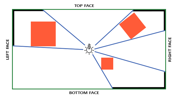
The shadow map we need implies rendering the scene in all directions around the light source and the usual 2D texture is not suitable here. So maybe use a cubic card ? Since a cubic map can store environmental data with just six faces, you can draw the entire scene onto each of these faces and then select a depth from the cube map.


The created cubic shadow map eventually ends up in a fragmentary shader, where it is sampled from it using the direction vector to obtain the fragment depth value (from the point of view of the source). Most of the technically complex parts we have already discussed in the previous lesson, so there remains one subtlety - the use of a cube map.

Create a cubic map

To create a cube map that stores the depth values ​​of the light source, we need to render the scene six times: once for each edge of the map. One of the (obvious) ways to accomplish this is to simply draw the scene six times, using six different viewports, and connecting a separate face of the cube map to each color attachment of the frame buffer object:

for(unsigned int i = 0; i < 6; i++) { GLenum face = GL_TEXTURE_CUBE_MAP_POSITIVE_X + i; glFramebufferTexture2D(GL_FRAMEBUFFER, GL_DEPTH_ATTACHMENT, face, depthCubemap, 0); BindViewMatrix(lightViewMatrices[i]); RenderScene(); } 

This approach can be very costly in performance, since many draw calls are made to create a single shadow map. In the lesson, we will try to implement a more optimal approach, using a small trick associated with using a geometric shader. This will create a cubic depth map in just one pass.

First create a cubic map:

 unsigned int depthCubemap; glGenTextures(1, &depthCubemap); 

And we define each face as a 2D texture that stores the depth values:

 const unsigned int SHADOW_WIDTH = 1024, SHADOW_HEIGHT = 1024; glBindTexture(GL_TEXTURE_CUBE_MAP, depthCubemap); for (unsigned int i = 0; i < 6; ++i) glTexImage2D(GL_TEXTURE_CUBE_MAP_POSITIVE_X + i, 0, GL_DEPTH_COMPONENT, SHADOW_WIDTH, SHADOW_HEIGHT, 0, GL_DEPTH_COMPONENT, GL_FLOAT, NULL); 

Also, do not forget to set the appropriate texture parameters:

 glTexParameteri(GL_TEXTURE_CUBE_MAP, GL_TEXTURE_MAG_FILTER, GL_NEAREST); glTexParameteri(GL_TEXTURE_CUBE_MAP, GL_TEXTURE_MIN_FILTER, GL_NEAREST); glTexParameteri(GL_TEXTURE_CUBE_MAP, GL_TEXTURE_WRAP_S, GL_CLAMP_TO_EDGE); glTexParameteri(GL_TEXTURE_CUBE_MAP, GL_TEXTURE_WRAP_T, GL_CLAMP_TO_EDGE); glTexParameteri(GL_TEXTURE_CUBE_MAP, GL_TEXTURE_WRAP_R, GL_CLAMP_TO_EDGE); 

In the usual approach, we would connect each face of the cube map to the frame buffer and render the scene six times, replacing the face of the cube map connected to attaching the frame buffer depth in each pass. But using the geometric shader, we can bring the scene to all faces at once in one pass, and therefore connect the cubic map directly to the depth attachment:

 glBindFramebuffer(GL_FRAMEBUFFER, depthMapFBO); glFramebufferTexture(GL_FRAMEBUFFER, GL_DEPTH_ATTACHMENT, depthCubemap, 0); glDrawBuffer(GL_NONE); glReadBuffer(GL_NONE); glBindFramebuffer(GL_FRAMEBUFFER, 0); 

Again, I’ll note the calls to glDrawBuffer and glReadBuffer : since only the depth values ​​are important to us, we explicitly tell OpenGL not to write to the color buffer.
In the end, two passes will be applied here: the shadow map is prepared first, the scene is drawn second, and the map is used to create shading. Using the framebuffer and the cube map, the code looks like this:

 // 1.      glViewport(0, 0, SHADOW_WIDTH, SHADOW_HEIGHT); glBindFramebuffer(GL_FRAMEBUFFER, depthMapFBO); glClear(GL_DEPTH_BUFFER_BIT); ConfigureShaderAndMatrices(); RenderScene(); glBindFramebuffer(GL_FRAMEBUFFER, 0); // 2.           glViewport(0, 0, SCR_WIDTH, SCR_HEIGHT); glClear(GL_COLOR_BUFFER_BIT | GL_DEPTH_BUFFER_BIT); ConfigureShaderAndMatrices(); glBindTexture(GL_TEXTURE_CUBE_MAP, depthCubemap); RenderScene(); 

In the first approximation, the process is the same as when using directional shadow maps. The only difference is that we render to a cubic depth map, and not to the usual 2D texture.

Before we proceed to direct rendering of the scene from the directions, relative to the source, we need to prepare suitable transformation matrices.

Conversion to a light source coordinate system

Having a prepared frame buffer object and a cubic map, we turn to the question of transforming all the objects of the scene into coordinate spaces corresponding to all six directions from the light source. We will create transformation matrices in the same way as in the previous lesson , but this time we will need a separate matrix for each face.

Each final transformation to the source space contains both a projection matrix and a view matrix. For the projection matrix, we use the perspective projection matrix: the source is a point in space, so the perspective projection here is most suitable. This matrix will be the same for all final conversions:

 float aspect = (float)SHADOW_WIDTH/(float)SHADOW_HEIGHT; float near = 1.0f; float far = 25.0f; glm::mat4 shadowProj = glm::perspective(glm::radians(90.0f), aspect, near, far); 

I note an important point: the parameter of the viewing angle when forming the matrix is ​​set to 90 °. It is this value of the viewing angle that provides us with a projection that allows us to correctly fill the faces of the cube map so that they converge without gaps.

Since the projection matrix remains constant, the same matrix can be reused to create all six final transformation matrices. But species matrices are needed unique for each face. Using glm :: lookAt we will create six matrices representing six directions in the following order: right, left, up, down, near edge, far edge:

 std::vector<glm::mat4> shadowTransforms; shadowTransforms.push_back(shadowProj * glm::lookAt(lightPos, lightPos + glm::vec3( 1.0, 0.0, 0.0), glm::vec3(0.0,-1.0, 0.0)); shadowTransforms.push_back(shadowProj * glm::lookAt(lightPos, lightPos + glm::vec3(-1.0, 0.0, 0.0), glm::vec3(0.0,-1.0, 0.0)); shadowTransforms.push_back(shadowProj * glm::lookAt(lightPos, lightPos + glm::vec3( 0.0, 1.0, 0.0), glm::vec3(0.0, 0.0, 1.0)); shadowTransforms.push_back(shadowProj * glm::lookAt(lightPos, lightPos + glm::vec3( 0.0,-1.0, 0.0), glm::vec3(0.0, 0.0,-1.0)); shadowTransforms.push_back(shadowProj * glm::lookAt(lightPos, lightPos + glm::vec3( 0.0, 0.0, 1.0), glm::vec3(0.0,-1.0, 0.0)); shadowTransforms.push_back(shadowProj * glm::lookAt(lightPos, lightPos + glm::vec3( 0.0, 0.0,-1.0), glm::vec3(0.0,-1.0, 0.0)); 

In the above code, the six created species matrices are multiplied by the projection matrix to specify the six unique matrices that transform into the light source space. The target parameter in the call to glm :: lookAt is the direction of looking at each of the faces of the cube map.

Further, this list of matrices is transmitted to the shaders when rendering a cubic depth map.

Depth recording shaders

To record the depth in a cubic map, we use three shaders: a vertex, a fragment, and an additional geometric one, which is executed between these stages.

It is the geometric shader that will be responsible for transforming all the vertices in world space into six separate spaces of the light source. Thus, the vertex shader is trivial and simply gives the coordinates of the vertex in world space, which will go to the geometric shader:

 #version 330 core layout (location = 0) in vec3 aPos; uniform mat4 model; void main() { gl_Position = model * vec4(aPos, 1.0); } 

The geometric shader accepts three vertices of the triangle as well as uniforms with an array of matrixes of transformation into the light source space. Here lies an interesting point: it is the geometric shader that will deal with converting vertices from world coordinates into source spaces.

For the geometry shader, the built-in variable gl_Layer is available , which specifies the face number of the cube map for which the shader will form the primitive. Normally, the shader simply sends all primitives further to the pipeline without additional actions. But by changing the value of this variable, we can control which side of the cube map we are going to render each of the primitives being processed. Of course, this only works if a cubic map is connected to the frame buffer.

 #version 330 core layout (triangles) in; layout (triangle_strip, max_vertices=18) out; uniform mat4 shadowMatrices[6]; //  FragPos     //      EmitVertex() out vec4 FragPos; void main() { for(int face = 0; face < 6; ++face) { //  ,    //      gl_Layer = face; for(int i = 0; i < 3; ++i) //      { FragPos = gl_in[i].gl_Position; gl_Position = shadowMatrices[face] * FragPos; EmitVertex(); } EndPrimitive(); } } 

The code presented should be pretty straightforward. The shader receives a primitive type triangle at the input, and as a result produces six triangles (6 * 3 = 18 vertices). In the main function, we loop through all six faces of the cube map, setting the current index as the number of the active face of the cube map with the corresponding entry in the gl_Layer variable. We also transform each input vertex from the world coordinate system into the space of the light source corresponding to the current face of the cubic art. To do this, FragPos is multiplied by a suitable transformation matrix from the uniformal shadowMatrices . Note that the FragPos value is also passed to the fragment shader to calculate the fragment depth.

In the last lesson, we used an empty fragmentary shader, and OpenGL itself was busy calculating the depth for the shadow map. This time we will manually form a linear depth value, taking as a basis the distance between the position of the fragment and the light source. This calculation of the depth value makes subsequent shading calculations a little more intuitive.

 #version 330 core in vec4 FragPos; uniform vec3 lightPos; uniform float far_plane; void main() { //       float lightDistance = length(FragPos.xyz - lightPos); //    [0, 1]    far_plane lightDistance = lightDistance / far_plane; //       gl_FragDepth = lightDistance; } 

The fragment FragPos from the geometric shader, the source position vector, and the distance to the far clipping plane of the pyramid of the light source projection are placed at the input of the fragment shader. In this code, we simply calculate the distance between the fragment and the source, we reduce it to the range of values ​​[0., 1.] and write it as the result of the shader.

A render of a scene with these shaders and a cubic card connected to the frame buffer object should generate a fully prepared shadow map for use in the next render pass.

Omnidirectional shadow maps

Once we have everything prepared, we can proceed to the immediate rendering of the omnidirectional shadows. The procedure is similar to that presented in the previous lesson for directional shadows, but this time we use a cubic texture instead of a two-dimensional one as a depth map, and also transfer uniforms with the far plane value of the projection pyramid for the light source to shaders.

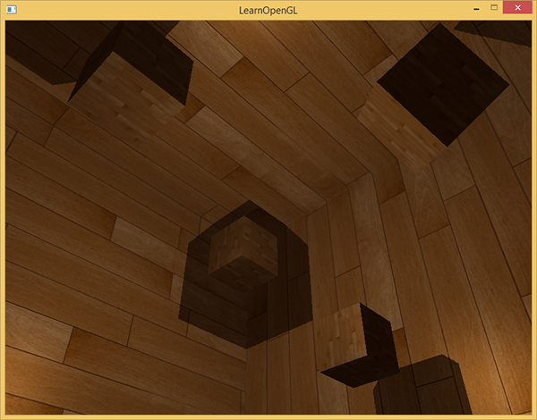
 glViewport(0, 0, SCR_WIDTH, SCR_HEIGHT); glClear(GL_COLOR_BUFFER_BIT | GL_DEPTH_BUFFER_BIT); shader.use(); // ...      (      far_plane) glActiveTexture(GL_TEXTURE0); glBindTexture(GL_TEXTURE_CUBE_MAP, depthCubemap); // ...   RenderScene(); 

In the example, the renderScene function displays several cubes located in a large cubic room that will cast shadows from a light source located in the center of the scene.

The summit and fragment shaders are almost identical to those considered in the lesson in directional shadows. So, in the fragment shader, the input parameter of the fragment position in the light source space is no longer required, since the selection from the shadow map is now done using the direction vector.

The vertex shader, accordingly, now does not have to convert the position vector to the light source space, so we can throw out the FragPosLightSpace variable:

 #version 330 core layout (location = 0) in vec3 aPos; layout (location = 1) in vec3 aNormal; layout (location = 2) in vec2 aTexCoords; out vec2 TexCoords; out VS_OUT { vec3 FragPos; vec3 Normal; vec2 TexCoords; } vs_out; uniform mat4 projection; uniform mat4 view; uniform mat4 model; void main() { vs_out.FragPos = vec3(model * vec4(aPos, 1.0)); vs_out.Normal = transpose(inverse(mat3(model))) * aNormal; vs_out.TexCoords = aTexCoords; gl_Position = projection * view * model * vec4(aPos, 1.0); } 

The code for the Blinna-Phong lighting model in the fragment shader remains intact, and it also leaves the multiplication by the shading factor at the end:

 #version 330 core out vec4 FragColor; in VS_OUT { vec3 FragPos; vec3 Normal; vec2 TexCoords; } fs_in; uniform sampler2D diffuseTexture; uniform samplerCube depthMap; uniform vec3 lightPos; uniform vec3 viewPos; uniform float far_plane; float ShadowCalculation(vec3 fragPos) { [...] } void main() { vec3 color = texture(diffuseTexture, fs_in.TexCoords).rgb; vec3 normal = normalize(fs_in.Normal); vec3 lightColor = vec3(0.3); //   vec3 ambient = 0.3 * color; //   vec3 lightDir = normalize(lightPos - fs_in.FragPos); float diff = max(dot(lightDir, normal), 0.0); vec3 diffuse = diff * lightColor; //   vec3 viewDir = normalize(viewPos - fs_in.FragPos); vec3 reflectDir = reflect(-lightDir, normal); float spec = 0.0; vec3 halfwayDir = normalize(lightDir + viewDir); spec = pow(max(dot(normal, halfwayDir), 0.0), 64.0); vec3 specular = spec * lightColor; //   float shadow = ShadowCalculation(fs_in.FragPos); vec3 lighting = (ambient + (1.0 - shadow) * (diffuse + specular)) * color; FragColor = vec4(lighting, 1.0); } 

I will also note a few subtle differences: the lighting model code is really unchanged, but now a sampler of the samplerCubemap type is used , and the ShadowCalculation function takes the coordinates of the fragment in world coordinates, instead of the light source space. We also use the pyramid parameter of the far_plane light source projection in further calculations. At the end of the shader, we calculate the shading factor, which is 1 when the fragment is in the shadow; or 0 when the fragment is outside the shadow. This coefficient is used to influence the prepared values ​​of the diffuse and specular components of the illumination.

The biggest changes relate to the body of the ShadowCalculation function, where the depth value is now sampled from a cube map, rather than a 2D texture. Let's sort the code of this function in order.

The first step is to get the immediate depth value from the cube map. As you remember, when preparing a cubic map, we wrote down the depth in it, represented as the distance between the fragment and the light source. The same approach is used here:

 float ShadowCalculation(vec3 fragPos) { vec3 fragToLight = fragPos - lightPos; float closestDepth = texture(depthMap, fragToLight).r; } 

The difference vector between the position of the fragment and the light source is calculated, which is used as the direction vector for the sample from the cube map. As we remember, the sampling vector from a cubic map does not have to be of unit length, then there is no need to normalize it. The obtained value of closestDepth is the normalized value of the depth of the nearest visible fragment relative to the light source.

Since the value of closestDepth is enclosed in the interval [0., 1.], then you should first perform the inverse transformation in the interval [0., far_plane ]:

 closestDepth *= far_plane; 

Next, we get the depth value for the current fragment relative to the light source. For the chosen approach, this is extremely simple: you only need to calculate the length of the already prepared vector fragToLight :

 float currentDepth = length(fragToLight); 

Thus, we obtain the depth value that lies in the same (or, perhaps, in a larger) interval as the closestDepth .

Now we can proceed to the comparison of both depth values ​​in order to find out if the current fragment is in the shadow or not. We also immediately include the offset value in the comparison in order not to encounter the problem of “shadow ripples” explained in the previous lesson :

 float bias = 0.05; float shadow = currentDepth - bias > closestDepth ? 1.0 : 0.0; 

Full ShadowCalculation Code:

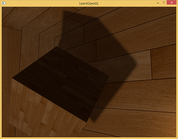
 float ShadowCalculation(vec3 fragPos) { //          vec3 fragToLight = fragPos - lightPos; //        //        float closestDepth = texture(depthMap, fragToLight).r; //       [0,1] //       closestDepth *= far_plane; //        //        float currentDepth = length(fragToLight); //   float bias = 0.05; float shadow = currentDepth - bias > closestDepth ? 1.0 : 0.0; return shadow; } 

With the given shaders, the application already displays quite tolerable shadows and this time they are dropped to all sides from the source. For a scene with a source in the center, the picture appears as follows:



The full source code is here .

Visualization of a cubic depth map

If you are somewhat similar to me, then, I think, you will not be able to do everything right the first time, and therefore some means of debugging the application would be quite useful. As the most obvious option, it would be nice to be able to verify the correctness of the preparation of the depth map. Since we now use a cubic map, rather than a two-dimensional texture, the question of visualization requires a somewhat more elaborate approach.

A simple solution would be to take the normalized value of closestDepth from the body of the ShadowCalculation function and output it as the result of a fragment shader:

 FragColor = vec4(vec3(closestDepth / far_plane), 1.0); 

The result is a scene in grayscale, where the intensity of the color corresponds to the linear depth value in the scene:


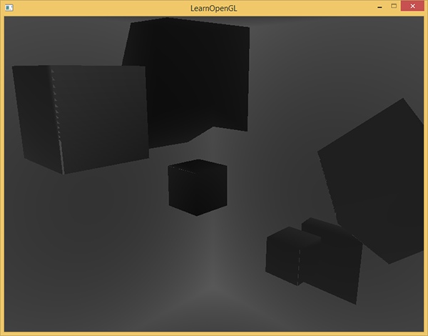
Also visible areas of shading on the walls of the room. If the result of visualization is similar to the above, then you can be sure that shadow maps have been prepared correctly. Otherwise, an error somewhere crept in: for example, the value of closestDepth was taken from the interval [0., far_plane ].

Percentage-closer filtering

Since omnidirectional shadows are built on the same principles as directed shadows, they inherited all the artifacts associated with the accuracy and finiteness of texture resolution. If you approach the borders of the shaded areas, the jagged edges become visible, i.e. aliasing artifacts. Percentage-closer filtering ( PCF ) filtering allows you to smooth out the aliasing traces by filtering multiple depth samples around the current fragment and averaging the result of depth comparison.

Take the PCF code from the previous lesson and add the third dimension (sampling from a cube map because it requires a direction vector):

 float shadow = 0.0; float bias = 0.05; float samples = 4.0; float offset = 0.1; for(float x = -offset; x < offset; x += offset / (samples * 0.5)) { for(float y = -offset; y < offset; y += offset / (samples * 0.5)) { for(float z = -offset; z < offset; z += offset / (samples * 0.5)) { float closestDepth = texture(depthMap, fragToLight + vec3(x, y, z)).r; closestDepth *= far_plane; //     [0;1] if(currentDepth - bias > closestDepth) shadow += 1.0; } } } shadow /= (samples * samples * samples); 

Little difference. We calculate the displacements for texture coordinates dynamically, based on the number of samples that we want to do along each axis and average the result by dividing by the number of samples raised to a cube.

Now the shadows look much more reliable and their edges are quite smooth.


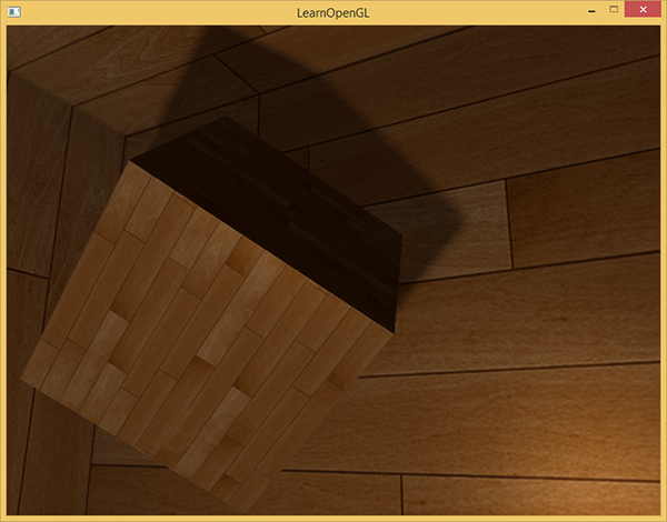
However, by setting the number of samples = 4 , we actually spend as many as 64 samples on each fragment, which is a lot.

And in most cases, these samples will be redundant, since they will be very close to the original vector of the sample. It would probably be more useful to do samples in directions perpendicular to the original vector of the sample. Alas, a simple method for finding out which of the generated additional directions will be redundant does not exist. You can use one technique and set an array of directions of displacement, all of which are almost completely separable vectors, i.e. each of them will point in completely different directions. This will reduce the number of directions of displacement, which will be too close to each other. Below is just a similar array with twenty specially selected directions of displacement:

 vec3 sampleOffsetDirections[20] = vec3[] ( vec3( 1, 1, 1), vec3( 1, -1, 1), vec3(-1, -1, 1), vec3(-1, 1, 1), vec3( 1, 1, -1), vec3( 1, -1, -1), vec3(-1, -1, -1), vec3(-1, 1, -1), vec3( 1, 1, 0), vec3( 1, -1, 0), vec3(-1, -1, 0), vec3(-1, 1, 0), vec3( 1, 0, 1), vec3(-1, 0, 1), vec3( 1, 0, -1), vec3(-1, 0, -1), vec3( 0, 1, 1), vec3( 0, -1, 1), vec3( 0, -1, -1), vec3( 0, 1, -1) ); 

, PCF sampleOffsetDirections . , , .

 float shadow = 0.0; float bias = 0.15; int samples = 20; float viewDistance = length(viewPos - fragPos); float diskRadius = 0.05; for(int i = 0; i < samples; ++i) { float closestDepth = texture(depthMap, fragToLight + sampleOffsetDirections[i] * diskRadius).r; closestDepth *= far_plane; //     [0;1] if(currentDepth - bias > closestDepth) shadow += 1.0; } shadow /= float(samples); 

diskRadius , , fragToLight .

: diskRadius . , :

 float diskRadius = (1.0 + (viewDistance / far_plane)) / 25.0; 

PCF , , :


, bias , , . , .

.

, , . , . , . , , , , , . , , . , .

Additional materials:

• Shadow Mapping for point light sources in OpenGL : sunandblackcat .
• Multipass Shadow Mapping With Point Lights : , ogldev .
• Omni-directional Shadows : , , Peter Houska .

PS : - . , !