Setting up a machine learning model: feature selection and optimization of hyper parameters

Introduction

In the previous article of the cycle, we discussed the formulation of the problem of data analysis, took the first steps in setting up a machine learning model, and wrote an interface suitable for use by an application programmer. Today we will conduct further research of the task - we will experiment with new signs, try more complex models and options for their tuning parameters.



As far as possible, the article uses Russian-language terminology chosen by the author on the basis of literal translations of English-language terms and established slang in the community. You can read about it here .

Recall what we stopped in terms of setting up the model and assessing the quality of its prediction on a validation sample.
')

We selected several signs describing the objects on which we teach our algorithm (and this, I remind you, such a boring and, it would seem, far from IT thing as industrial pipes). Based on these features, the key function to_sample() works, which currently looks like this:

 def to_sample(instance, additional_data): return (is_bracket_pricing(instance) + get_quantity(instance) + get_min_order_quantity(instance) + get_annual_usage(instance) + get_absolute_date(instance) + get_supplier(instance) + get_assembly_specs(instance, additional_data['assembly_to_specs'])) 

At the input, it takes a description of the object (the instance variable) contained in the main file train_set.csv and a set of additional data generated based on the remaining files from the dataset, and returns a fixed-length array at the output, which later goes to the input of the machine learning algorithm.

Regarding specific modeling, no particular progress has yet occurred - elementary linear regression is still used without any settings that differ from the default Scikit-Learn package. Nevertheless, for the time being we will continue to gradually increase the list of signs to improve the quality of the prediction algorithm. Last time, we already (in a rather, in a banal way) used all the columns of the main file with training data train_set.csv and the file with auxiliary data specs.csv . So now, perhaps, it is time to pay attention to the other files with additional data. In particular, the content of the bill_of_materials.csv file, which describes the components of each product, looks promising.

Further selection of signs

 $ head ./data/competition_data/bill_of_materials.csv tube_assembly_id,component_id_1,quantity_1,component_id_2,quantity_2,component_id_3,quantity_3,component_id_4,quantity_4,component_id_5,quantity_5,component_id_6,quantity_6,component_id_7,quantity_7,component_id_8,quantity_8 TA-00001,C-1622,2,C-1629,2,NA,NA,NA,NA,NA,NA,NA,NA,NA,NA,NA,NA TA-00002,C-1312,2,NA,NA,NA,NA,NA,NA,NA,NA,NA,NA,NA,NA,NA,NA TA-00003,C-1312,2,NA,NA,NA,NA,NA,NA,NA,NA,NA,NA,NA,NA,NA,NA TA-00004,C-1312,2,NA,NA,NA,NA,NA,NA,NA,NA,NA,NA,NA,NA,NA,NA TA-00005,C-1624,1,C-1631,1,C-1641,1,NA,NA,NA,NA,NA,NA,NA,NA,NA,NA TA-00006,C-1624,1,C-1631,1,C-1641,1,NA,NA,NA,NA,NA,NA,NA,NA,NA,NA TA-00007,C-1622,2,C-1629,2,NA,NA,NA,NA,NA,NA,NA,NA,NA,NA,NA,NA TA-00008,C-1312,2,NA,NA,NA,NA,NA,NA,NA,NA,NA,NA,NA,NA,NA,NA TA-00009,C-1625,2,C-1632,2,NA,NA,NA,NA,NA,NA,NA,NA,NA,NA,NA,NA 

As you can see, the file format resembles specs.csv . To begin with, let's see how many kinds of components are actually found, and already with the help of this information we will make a decision on what sign it is reasonable to form based on these auxiliary data.

 >>> set_of_components = set() >>> with open('./data/competition_data/bill_of_materials.csv') as input_stream: ... header_line = input_stream.readline() ... for line in input_stream: ... for i in range(1, 16, 2): ... new_component = line.split(',')[i] ... set_of_components.add(new_component) ... >>> len(set_of_components) 2049 >>> sorted(set_of_components)[:10] ['9999', 'C-0001', 'C-0002', 'C-0003', 'C-0004', 'C-0005', 'C-0006', 'C-0007', 'C-0008', 'C-0009'] 

The component turned out to be quite a few, so the idea of ​​deploying the attribute to an array of more than 2000 elements in a standard way does not seem very reasonable. Let's try to use several dozen of the most popular options, and also leave the variable responsible for the number of these variations as a tuning parameter for optimization at the fine tuning stage.

 def load_additional_data(): result = dict() ... assembly_to_components = dict() component_to_popularity = dict() with open('./data/competition_data/bill_of_materials.csv') as input_stream: header_line = input_stream.readline() for line in input_stream: tube_assembly_id = line.split(',')[0] assembly_to_components[tube_assembly_id] = dict() for i in range(1, 16, 2): new_component = line.split(',')[i] if new_component != 'NA': quantity = int(line.split(',')[i + 1]) assembly_to_components[tube_assembly_id][new_component] = quantity if new_component in component_to_popularity: component_to_popularity[new_component] += 1 else: component_to_popularity[new_component] = 1 components_by_popularity = [value[0] for value in sorted( component_to_popularity.items(), key=operator.itemgetter(1, 0), reverse=True)] result['assembly_to_components'] = assembly_to_components result['components_by_popularity'] = components_by_popularity ... def get_assembly_components(instance, assembly_to_components, components_by_popularity, number_of_components): """ number_of_components: number of most popular components taken into account """ result = [0] * number_of_components for component in sorted(assembly_to_components[instance['tube_assembly_id']]): component_index = components_by_popularity.index(component) if component_index < number_of_components: # quantity result[component_index] = assembly_to_components[ instance['tube_assembly_id']][component] return result def to_sample(instance, additional_data): return (is_bracket_pricing(instance) + get_quantity(instance) + get_min_order_quantity(instance) + get_annual_usage(instance) + get_absolute_date(instance) + get_supplier(instance) + get_assembly_specs(instance, additional_data['assembly_to_specs']) + get_assembly_components(instance, additional_data['assembly_to_components'], additional_data['components_by_popularity'], 100) ) 

Run the program without a new feature to remember what the result was on validation.

Mean Squared Error: 0.7754770419953809

And now add a new sign.

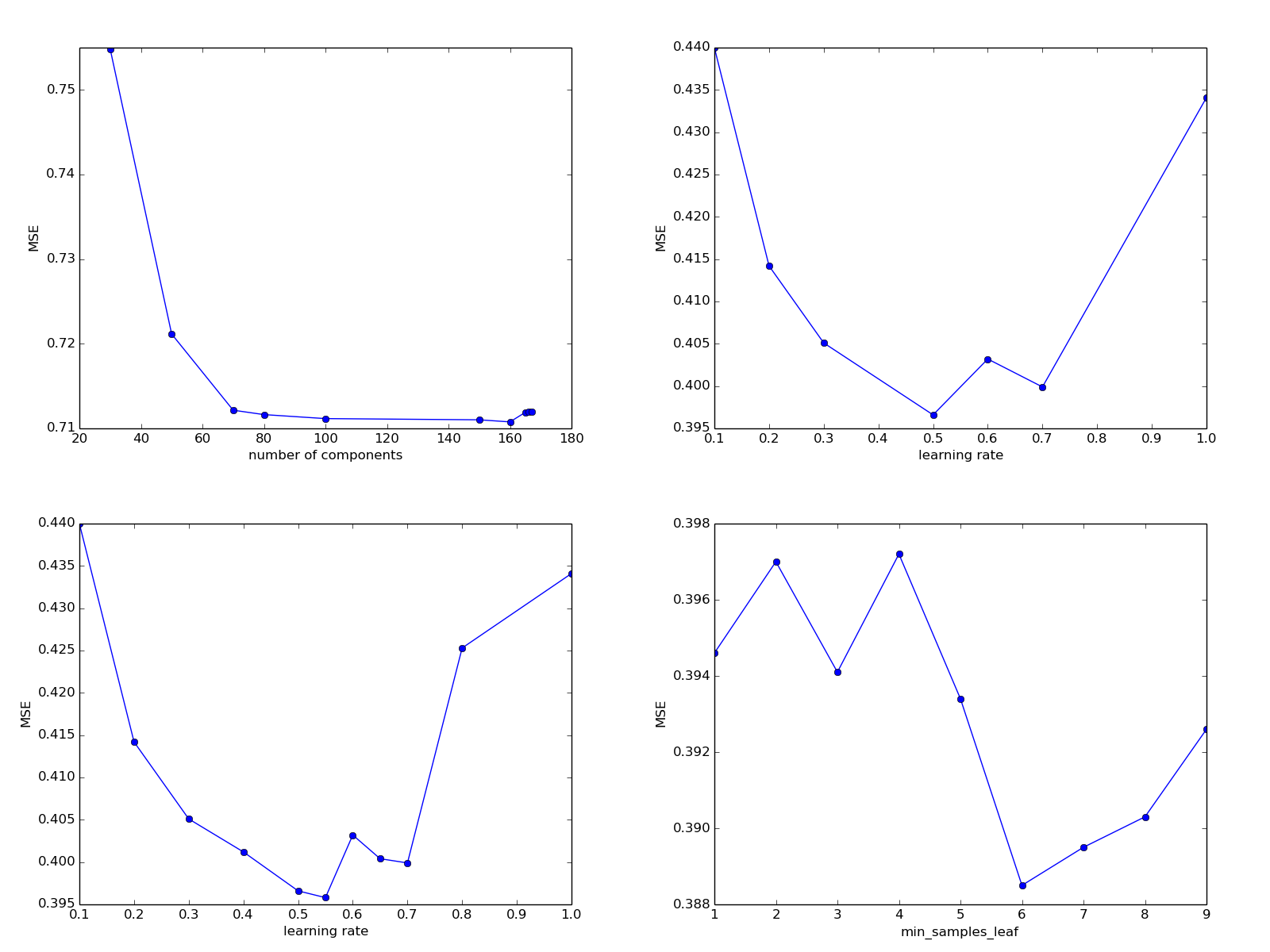
Mean Squared Error: 0.711158610883329

As we see, the quality of the prediction has again increased significantly. By the way, we have the first numerical tuning parameter, namely, the number of the most popular components that we take into account. Let's try to vary it, bearing in mind that, based on general considerations, as the parameter increases, the quality of the prediction should improve - after all, we take into account more and more previously unused information.

100: 0.711158610883329
200: 16433833.592963027
150: 0.7110152873760721
170: 19183113.422557358
160: 0.7107685953594116
165: 0.7119011633609398
168: 24813512.02303443
166: 0.7119603793730067
167: 0.7119604617354474

While it is difficult to say what happens after the disaster exceeds the value of 168, for what reason the quality of the prediction is so sharply and suddenly deteriorating. For the rest - we do not see any significant changes. To clear our conscience, let us see how the quality of the prediction will change with a decrease in the variable parameter.

80: 0.7116311373463766
50: 0.7211560841347712
30: 0.7548570148032887
70: 0.7121518708790175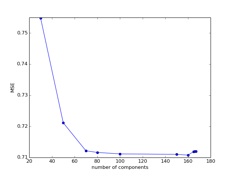



It can be seen that with a decrease in the number of components, the error increases, and for values ​​between 80 and 160, it remains approximately constant. Let's leave the parameter at 100 for now.

As you can see, adding new features still gives significant improvements on validation. We will conduct a couple more experiments of this kind and then proceed to varying the training models and their tuning parameters. Let us consider more complex, but, judging by the description of the data files, the key file is tube.csv .

 $ head data/competition_data/tube.csv tube_assembly_id,material_id,diameter,wall,length,num_bends,bend_radius,end_a_1x,end_a_2x,end_x_1x,end_x_2x,end_a,end_x,num_boss,num_bracket,other TA-00001,SP-0035,12.7,1.65,164,5,38.1,N,N,N,N,EF-003,EF-003,0,0,0 TA-00002,SP-0019,6.35,0.71,137,8,19.05,N,N,N,N,EF-008,EF-008,0,0,0 TA-00003,SP-0019,6.35,0.71,127,7,19.05,N,N,N,N,EF-008,EF-008,0,0,0 TA-00004,SP-0019,6.35,0.71,137,9,19.05,N,N,N,N,EF-008,EF-008,0,0,0 TA-00005,SP-0029,19.05,1.24,109,4,50.8,N,N,N,N,EF-003,EF-003,0,0,0 TA-00006,SP-0029,19.05,1.24,79,4,50.8,N,N,N,N,EF-003,EF-003,0,0,0 TA-00007,SP-0035,12.7,1.65,202,5,38.1,N,N,N,N,EF-003,EF-003,0,0,0 TA-00008,SP-0039,6.35,0.71,174,6,19.05,N,N,N,N,EF-008,EF-008,0,0,0 TA-00009,SP-0029,25.4,1.65,135,4,63.5,N,N,N,N,EF-003,EF-003,0,0,0 

Note that the contents of the “material_id” column match the prefix with the values ​​specified in specs.csv . What it means is difficult to say, and after conducting a search for several values ​​of the type SP-xyzt contained in the first 20 lines of specs.csv we will not find anything, but it's worth remembering this feature just in case. Also, based on the description of the competition, it is difficult to understand the actual difference between the material indicated in the column and the materials indicated in bill_of_materials.csv . We will not, however, so far torment ourselves with such tricky questions and try to analyze in the usual way the number of possible options and convert the value into (hopefully) a feature useful for the algorithm.

 >>> set_of_materials = set() >>> with open('./data/competition_data/tube.csv') as input_stream: ... header_line = input_stream.readline() ... for line in input_stream: ... new_material = line.split(',')[1] ... set_of_materials.add(new_material) ... >>> len(set_of_materials) 20 >>> set_of_materials {'SP-0034', 'SP-0037', 'SP-0039', 'SP-0030', 'SP-0029', 'NA', 'SP-0046', 'SP-0028', 'SP-0031', 'SP-0032', 'SP-0033', 'SP-0019', 'SP-0048', 'SP-0008', 'SP-0045', 'SP-0035', 'SP-0044', 'SP-0036', 'SP-0041', 'SP-0038'} 

It turned out quite a number of options, so that we can not hesitate to add a standard categorical feature. To do this, we first load_additional_data() function by loading the assembly_to_material dictionary.

 assembly_to_material = dict() with open('./data/competition_data/tube.csv') as input_stream: header_line = input_stream.readline() for line in input_stream: tube_assembly_id = line.split(',')[0] material_id = line.split(',')[1] assembly_to_material[tube_assembly_id] = material_id result['assembly_to_material'] = assembly_to_material 

And we use it when writing similar to one of the existing functions.

 MATERIALS_LIST = ['NA', 'SP-0008', 'SP-0019', 'SP-0028', 'SP-0029', 'SP-0030', 'SP-0031', 'SP-0032', 'SP-0033', 'SP-0034', 'SP-0035', 'SP-0036', 'SP-0037', 'SP-0038', 'SP-0039', 'SP-0041', 'SP-0044', 'SP-0045', 'SP-0046', 'SP-0048'] def get_material(instance, assembly_to_material): material = assembly_to_material[instance['tube_assembly_id']] if material in MATERIALS_LIST: material_index = MATERIALS_LIST.index(material) result = [0] * material_index + [1] + [0] * (len(MATERIALS_LIST) - material_index - 1) else: result = [0] * len(MATERIALS_LIST) return result 

Mean Squared Error: 0.7187098083419174

Alas, this symptom did not help us improve the already existing result of approximately 0.711. But it does not matter - you can hope that our work will not be in vain and will help in setting up a more complex model. The next column in the same tube.csv file describes the diameter of the tube. Such a property of an object is called quantitative and is converted into a sign in the simplest and most natural way, namely, by taking a value. Of course, in some cases it may be useful to somehow normalize it or change it in some other way, but for the first attempt, you can do without it. Having written the code corresponding to this feature, which has become a familiar way,

 def get_diameter(instance, assembly_to_diameter): return [assembly_to_diameter[instance['tube_assembly_id']]] 

and adding it to the to_sample() function, we can get another improvement in the quality of model prediction on a validation sample.

Mean Squared Error: 0.6968043166687439

As we see, simple extraction of new and new features and testing the quality of model prediction on a validation sample continues to improve the quality metric. However, on the one hand, the increase in new signs is no longer so great (and sometimes negative - and then the corresponding attribute must be abandoned, as in the previous example with the material), and on the other, we have a training project, not a competitive or working one. , so let's leave for the time the selection of features and move on to the question of choosing the algorithm and optimizing the parameters.

We vary models

In the framework of the current set of features, we will try to find a machine learning model that is close to optimal and has a corresponding set of hyper parameters. Let's start with testing different models. Let's try to replace the simplest linear regression with a fashionable neural net from the Keras package, one of the easiest to use.

 from keras.models import Sequential from keras.layers import Dense from keras.optimizers import SGD model = Sequential() model.add(Dense(units=30, activation='tanh', input_dim=len(list_of_samples[0]))) model.add(Dense(units=1, activation='linear')) optimizer = SGD(lr=0.1) model.compile(loss='mean_squared_error', optimizer=optimizer, metrics=['accuracy']) 

That corresponds to the fully connected network architecture with the number of neurons in the layer equal to 30, learning_rate equal to 0.1 and activation function tanh . Note that at the output layer the function is linear, and not one or another variation of sigmoids, since we predict a numerical parameter.

Mean Squared Error: nan

The error turned out to be so great that it did not fit in the (very rather big) numpy-ev int. Let's try to add another layer.

 from keras.models import Sequential from keras.layers import Dense from keras.optimizers import SGD model = Sequential() model.add(Dense(units=30, activation='tanh', input_dim=len(list_of_samples[0]))) model.add(Dense(units=20, activation='tanh', input_dim=len(list_of_samples[0]))) model.add(Dense(units=1, activation='linear')) optimizer = SGD(lr=0.1) model.compile(loss='mean_squared_error', optimizer=optimizer, metrics=['accuracy']) 

Mean Squared Error: nan

Again, a good result did not work. It is a pity, but, apparently, neural networks are a useful and good model, but not for our task. However, if someone is able to get a good result for her using neural network type models, then I wait for references to the code in the comments, and we will switch to more conservative approaches. For example, one of the standard algorithms for solving a regression problem is gradient boosting. Let's try to use it.

 model = GradientBoostingRegressor() 

Mean Squared Error: 0.44000911792278125

Obvious great progress, no doubt lifted us up after a deafening failure with the advertised neural networks. Here, of course, you can try some other algorithm like RidgeRegression, but in general, the author already knew that the gradient boosting for such tasks fits well, neural networks are very bad, and the other models are more or less, so let's not go through all possible options, and we will be engaged in optimization of hyper parameters of the most suitable of them, namely boosting.

Going to the appropriate page of the Scikit-Learn website dedicated to the library, located here or simply typing help (GradientBoostingRegressor) in the console, we learn that this implementation of the algorithm has the following set of tuning parameters and their default values:

loss='ls'
learning_rate=0.1
n_estimators=100
subsample=1.0
criterion='friedman_mse'
min_samples_split=2
min_samples_leaf=1
min_weight_fraction_leaf=0.0
max_depth=3
min_impurity_decrease=0.0
min_impurity_split=None
init=None
random_state=None
max_features=None
alpha=0.9
verbose=0
max_leaf_nodes=None
warm_start=False
presort='auto'

Let's analyze them one by one and try changing the ones that, at first glance, can help improve the quality of the prediction.

  | loss : {'ls', 'lad', 'huber', 'quantile'}, optional (default='ls') | loss function to be optimized. 'ls' refers to least squares | regression. 'lad' (least absolute deviation) is a highly robust | loss function solely based on order information of the input | variables. 'huber' is a combination of the two. 'quantile' | allows quantile regression (use `alpha` to specify the quantile). 

The loss function that we optimize. It would seem that after our reformulation of the task (in terms of taking logarithms from labels and, accordingly, MSE optimization instead of LMSE), the default parameter corresponds to our task. Leave as is.

  | learning_rate : float, optional (default=0.1) | learning rate shrinks the contribution of each tree by `learning_rate`. | There is a trade-off between learning_rate and n_estimators. 

In many tasks, the key parameter to configure. Let's try to see what will happen for other values.

 MODEL_SETTINGS = { 'model_name':'GradientBoostingRegressor', 'learning_rate':0.100} ... model = GradientBoostingRegressor(learning_rate=MODEL_SETTINGS['learning_rate']) 

A simple explicit declaration of the hyperparameter is written in such a somewhat fanciful form so that in the future it would be convenient to change the parameters of the model (and the models themselves) in the script header, as well as for reasons of ease of logging.

Mean Squared Error: 0.44002379237806705

 MODEL_SETTINGS = { 'model_name':'GradientBoostingRegressor', 'learning_rate':0.200} 

Mean Squared Error: 0.41423518862618164

Aha, with an increase in learning_rate the quality metric improves significantly. Let's try to continue to change this parameter in the same direction.

 MODEL_SETTINGS = { 'model_name':'GradientBoostingRegressor', 'learning_rate':0.300} 

Mean Squared Error: 0.4051555356961356

Increase more

 MODEL_SETTINGS = { 'model_name':'GradientBoostingRegressor', 'learning_rate':0.500} 

Mean Squared Error: 0.39668129369369115

And further

 MODEL_SETTINGS = { 'model_name':'GradientBoostingRegressor', 'learning_rate':1.000} 

Mean Squared Error: 0.434184026080522

With the next increase in the parameter, the target metric has deteriorated. Let's try to look for something among intermediate values.

 MODEL_SETTINGS = { 'model_name':'GradientBoostingRegressor', 'learning_rate':0.700} 

Mean Squared Error: 0.39998809063954305

 MODEL_SETTINGS = { 'model_name':'GradientBoostingRegressor', 'learning_rate':0.600} 

Mean Squared Error: 0.4032676539076024

The data obtained in the experiments are already quite confusing, let's tabulate them and draw the corresponding schedule (I personally do not usually look at the graphs in such cases, limiting themselves to mental constructions, but for pedagogical purposes this may be useful).

learning_rate	MSE
0.100	0.4400
0.200	0.4142
0.300	0.4051
0.500	0.3966
0.600	0.4032
0.700	0.3999
1,000	0.4341

At first glance, it looks as if the quality metric improves with a decrease in learning_rate from 0.100 to 0.500, then, until approximately 0.700, it remains relatively stable, and then worsens. Let's test this hypothesis with more experiments.

 MODEL_SETTINGS = { 'model_name':'GradientBoostingRegressor', 'learning_rate':0.400} 

Mean Squared Error: 0.40129637223972486

 MODEL_SETTINGS = { 'model_name': 'GradientBoostingRegressor', 'learning_rate': 0.800} 

Mean Squared Error: 0.4253214442400451

 MODEL_SETTINGS = { 'model_name': 'GradientBoostingRegressor', 'learning_rate': 0.550} 

Mean Squared Error: 0.39587242367884334

 MODEL_SETTINGS = { 'model_name': 'GradientBoostingRegressor', 'learning_rate': 0.650} 

Mean Squared Error: 0.40041838873950636

learning_rate	MSE
0.100	0.4400
0.200	0.4142
0.300	0.4051
0.400	0.4012
0.500	0.3966
0.550	0.3958
0.600	0.4032
0.650	0.4004
0.700	0.3999
0.800	0.4253
1,000	0.4341

It seems that the optimal value lies somewhere around 0.500 - 0.550 and changes in one direction or another by and large already have little effect on the final metric compared to other possible changes in the parameters of the model or the list of features. Let's fix the learning_rate on the value 0.550 and pay attention to other parameters of our model.

By the way, in similar cases, in order to verify the correct selection of one or another set of hyperparameters, it may be useful to change the random_state parameter that many algorithms have or even divide the sample into training and validation while maintaining the number of elements in them. This will help to gather more information about the real efficiency of the algorithm in the case of not quite clear patterns between the settings of the hyperparameters and the quality of the prediction on the validation sample.

| n_estimators: int (default = 100)
| The number of boost stages to perform. Gradient boosting
| large number usually
| results in better performance.

The number of some “boosting stages” when learning a gradient boosting model. The author, to be frank, has already forgotten what role they play in the formal definition of the algorithm, however, let’s take this argument. By the way, let's begin to note the time spent on training the model.

 import time MODEL_SETTINGS = { 'model_name':'GradientBoostingRegressor', 'learning_rate':0.550, 'n_estimators':100} model = GradientBoostingRegressor(learning_rate=MODEL_SETTINGS['learning_rate'], n_estimators=MODEL_SETTINGS['n_estimators']) time_start = time.time() model.fit(numpy.array(train_samples), numpy.array(train_labels)) print('Time spent: {0}'.format(time.time() - time_start)) print('MODEL_SETTINGS = {{\n {0}\n {1}\n {2}}}' .format(MODEL_SETTINGS['model_name'], MODEL_SETTINGS['learning_rate'], MODEL_SETTINGS['n_estimators'])) 

 MODEL_SETTINGS = { 'model_name': GradientBoostingRegressor, 'learning_rate': 0.55, 'n_estimators': 100} 

Time spent: 71.83099746704102
Mean Squared Error: 0.39622103688045596

 MODEL_SETTINGS = { 'model_name': GradientBoostingRegressor 'learning_rate': 0.55 'n_estimators': 200} 

Time spent: 141.9290111064911
Mean Squared Error: 0.40527237378150016

, , . - .

 MODEL_SETTINGS = { 'model_name': GradientBoostingRegressor 'learning_rate': 0.55 'n_estimators': 300} 

Time spent: 204.2548701763153
Mean Squared Error: 0.4027642069054909

, , .

| max_depth: integer, optional (default=3)
| maximum depth of the individual regression estimators. The maximum
| depth limits the number of nodes in the tree. Tune this parameter
| for best performance; the best value depends on the interaction
| of the input variables.

 MODEL_SETTINGS = { 'model_name': GradientBoostingRegressor 'learning_rate': 0.55 'n_estimators': 100 'max_depth': 3} 

Time spent: 66.88031792640686
Mean Squared Error: 0.39713231957974565

 MODEL_SETTINGS = { 'model_name': GradientBoostingRegressor 'learning_rate': 0.55 'n_estimators': 100 'max_depth': 4} 

Time spent: 86.24338245391846
Mean Squared Error: 0.40575622943301354

 MODEL_SETTINGS = { 'model_name': GradientBoostingRegressor 'learning_rate': 0.55 'n_estimators': 100 'max_depth': 2} 

Time spent: 45.39022421836853
Mean Squared Error: 0.41356622455188463

, — .

| criterion: string, optional (default=«friedman_mse»)
| The function to measure the quality of a split. Supported criteria
| are «friedman_mse» for the mean squared error with improvement
| score by Friedman, «mse» for mean squared error, and «mae» for
| the mean absolute error. The default value of «friedman_mse» is
| generally the best as it can provide a better approximation in
| some cases.

, , - , , .

| min_samples_split: int, float, optional (default=2)
| The minimum number of samples required to split an internal node:
|
| — If int, then consider `min_samples_split` as the minimum number.
| — If float, then `min_samples_split` is a percentage and
| `ceil(min_samples_split * n_samples)` are the minimum
| number of samples for each split.
|
|… versionchanged:: 0.18
| Added float values for percentages.

, . .

 MODEL_SETTINGS = { 'model_name': GradientBoostingRegressor 'learning_rate': 0.55 'n_estimators': 100 'max_depth': 3 'min_samples_split': 2 } <source> <code>Time spent: 66.22262406349182</code> <code>Mean Squared Error: 0.39721489877049687</code>    - ,  ,      .  . <source lang="python"> MODEL_SETTINGS = { 'model_name': GradientBoostingRegressor, 'learning_rate': 0.55, 'n_estimators': 100, 'max_depth': 3 , 'min_samples_split': 3 } 

Time spent: 66.18473935127258
Mean Squared Error: 0.39493122173406714

 MODEL_SETTINGS = { 'model_name': GradientBoostingRegressor 'learning_rate': 0.55 'n_estimators': 100 'max_depth': 3 'min_samples_split': 8 } 

Time spent: 66.7643404006958
Mean Squared Error: 0.3982469042761572

, . 4.

 MODEL_SETTINGS = { 'model_name': GradientBoostingRegressor, 'learning_rate': 0.55, 'n_estimators': 100, 'max_depth': 3, 'min_samples_split': 4 } 

Time spent: 66.75952744483948
Mean Squared Error: 0.3945186290058591

- , 3, , , , , .

| min_samples_leaf: int, float, optional (default=1)
| The minimum number of samples required to be at a leaf node:
|
| — If int, then consider `min_samples_leaf` as the minimum number.
| — If float, then `min_samples_leaf` is a percentage and
| `ceil(min_samples_leaf * n_samples)` are the minimum
| number of samples for each node.
|
|… versionchanged:: 0.18
| Added float values for percentages.

, . (. . , ) , , . , , .

 MODEL_SETTINGS = { 'model_name': GradientBoostingRegressor, 'learning_rate': 0.55, 'n_estimators': 100, 'max_depth': 3, 'min_samples_split': 4 'min_samples_leaf': 1} 

Time spent: 68.58824563026428
Mean Squared Error: 0.39465027476703846

« » . , , ( ) , .

 MODEL_SETTINGS = { 'model_name': GradientBoostingRegressor, 'learning_rate': 0.55, 'n_estimators': 100, 'max_depth': 3, 'min_samples_split': 4 'min_samples_leaf': 2} 

Time spent: 68.03447198867798
Mean Squared Error: 0.39707533548242

1 2 . - .

 MODEL_SETTINGS = { 'model_name': GradientBoostingRegressor, 'learning_rate': 0.55, 'n_estimators': 100, 'max_depth': 3, 'min_samples_split': 4, 'min_samples_leaf': 3, 'random_seed': 0} 

Time spent: 66.98832631111145
Mean Squared Error: 0.39419555554861274

, , , , . , , . , random_seed.

 MODEL_SETTINGS = { 'model_name': GradientBoostingRegressor, 'learning_rate': 0.55, 'n_estimators': 100, 'max_depth': 3, 'min_samples_split': 4, 'min_samples_leaf': 3, 'random_seed': 1} 

Time spent: 67.16857171058655
Mean Squared Error: 0.39483997966302

 MODEL_SETTINGS = { 'model_name': GradientBoostingRegressor, 'learning_rate': 0.55, 'n_estimators': 100, 'max_depth': 3, 'min_samples_split': 4 'min_samples_leaf': 3, 'random_seed': 2} 

Time spent: 66.11015605926514
Mean Squared Error: 0.39492203941997045

, , . « » , . .

 MODEL_SETTINGS = { 'model_name': GradientBoostingRegressor, 'learning_rate': 0.55, 'n_estimators': 100, 'max_depth': 3, 'min_samples_split': 4 'min_samples_leaf': 4 , 'random_seed': 0} 

Time spent: 66.96864414215088
Mean Squared Error: 0.39725274882841366

. , , - , ? .

 MODEL_SETTINGS = { 'model_name': GradientBoostingRegressor, 'learning_rate': 0.55, 'n_estimators': 100, 'max_depth': 3, 'min_samples_split': 4 'min_samples_leaf': 5 , 'random_seed': 0} 

Time spent: 66.33412432670593
Mean Squared Error: 0.39348528600652666

 MODEL_SETTINGS = { 'model_name': GradientBoostingRegressor, 'learning_rate': 0.55, 'n_estimators': 100, 'max_depth': 3, 'min_samples_split': 4 'min_samples_leaf': 5 , 'random_seed': 1} 

Time spent: 66.22624254226685
Mean Squared Error: 0.3935675331843957

. «» . , .

 MODEL_SETTINGS = { 'model_name': GradientBoostingRegressor, 'learning_rate': 0.55, 'n_estimators': 100, 'max_depth': 3, 'min_samples_split': 4, 'min_samples_leaf': 6 , 'random_seed': 0} 

Time spent: 66.88769054412842
Mean Squared Error: 0.38855940004423717

5 6 . , .

min_samples_leaf	MSE	time spent
one	0.3946	68.58
2	0.3970	68.03
3	0.3941	66.98
four	0.3972	66.96
five	0.3934	66.33
6	0.3885	66.88
7	0.3895	65.22
eight	0.3903	65.89
9	0.3926	66.31

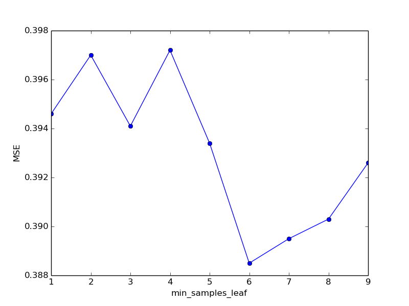
, , min_samples_leaf 6. .

| min_weight_fraction_leaf: float, optional (default=0.)
| The minimum weighted fraction of the sum total of weights (of all
| the input samples) required to be at a leaf node. Samples have
| equal weight when sample_weight is not provided.

, . , . , , mean_samples_leaf.

 MODEL_SETTINGS = { 'model_name': GradientBoostingRegressor, 'learning_rate': 0.55, 'n_estimators': 100, 'max_depth': 3, 'min_samples_split': 4, 'min_samples_leaf': 6 , 'random_seed': 0, 'min_weight_fraction_leaf': 0.01} 

Time spent: 68.06336092948914
Mean Squared Error: 0.41160143391833687

, . , ?

 MODEL_SETTINGS = { 'model_name': GradientBoostingRegressor, 'learning_rate': 0.55, 'n_estimators': 100, 'max_depth': 3, 'min_samples_split': 4, 'min_samples_leaf': 6 , 'random_seed': 0, 'min_weight_fraction_leaf': 0.001} 

Time spent: 67.03254532814026
Mean Squared Error: 0.39262469473669265

. , , , min_samples_leaf, min_weight_fraction_leaf. .

| subsample: float, optional (default=1.0)
| The fraction of samples to be used for fitting the individual base
| learners. If smaller than 1.0 this results in Stochastic Gradient
| Boosting. `subsample` interacts with the parameter `n_estimators`.
| Choosing `subsample < 1.0` leads to a reduction of variance
| and an increase in bias.

 MODEL_SETTINGS = { 'model_name': GradientBoostingRegressor, 'learning_rate': 0.55, 'n_estimators': 100, 'max_depth': 3, 'min_samples_split': 4, 'min_samples_leaf': 6, 'random_seed': 0, 'min_weight_fraction_leaf': 0.0, 'subsample': 0.9} 

Time spent: 155.24894833564758
Mean Squared Error: 0.39231319253775626

, ( , ). , , kaggle . , kaggle , , , , .

generate_response.py.


, research.py test_set.csv , , . output.csv . , generate_response.py (serving) . , , , , , , , .

kaggle , , .



, , — , . , , , — ( ) . .

Conclusion

, , , , , , , kaggle. , !