Measurement of fluid level in the rocket fuel tank

Introduction

The fuel from the oxidizer tank and the fuel tank enters the combustion chamber of the rocket engine. The synchronous supply of fuel in a given proportion ensures efficient operation of the rocket engine.

Efficient operation depends on accurate measurement of the fuel level in the tank. For this purpose, the fuel tank has a fuel management system. The system is a vertical measuring channel with sensors inside the channel for fixing the free liquid level in the channel [1]:
')

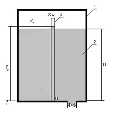
Picture. Fuel tank layout. 1- reservoir, 2- fuel, 3- measuring channel, Po - gas pressure, - liquid level in the channel, H - liquid level in the tank, r, x - coordinate axes.

The vertical channel and fuel tank are communicating vessels. By reducing the level of fuel in the tank, the level of fuel in the measuring channel decreases. When the fuel level in the channel reaches the sensor, the sensor is activated. The signal enters the fuel management system.

As a result, its fuel consumption in the tank changes. Thus, the level of fuel in the channel must determine the level of fuel in the tank. There are two problems. The first method is that the free surface of the fuel in the tank does not coincide with the surface of the fuel in the channel.

The second problem is level fluctuations when the rocket accelerates in flight, which leads to false positives of the sensors and, as a result, to measurement errors.

An error in measuring the fuel level leads to inefficient fuel consumption. As a result, the rocket engine does not work optimally, and “excess” fuel may remain in the tanks.

Next, we consider how to determine the methodological error from the first problem and reduce the measurement error from the second.

In order not to send the reader to the link [1], I will give here the derivation of the differential equation of fluid motion in the measuring channel, at the same time correcting mathematical and grammatical errors.

During flight t, the level of liquid H in the fuel tank changes according to the relation:

(one)

Where: –– initial fuel level in the tank; V– fuel rate of change.

With the introduced coordinate system (see figure), the equation for the unsteady motion of a viscous incompressible fluid in the measuring channel will be:

(2)

With boundary and primary conditions.

where: u (r, t) is the velocity of the fluid in the channel; p is pressure; ρ is the density; time - t; v is the kinematic viscosity; g- acceleration of gravity.

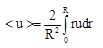
We obtain the ratio for the average speed in the measuring channel:

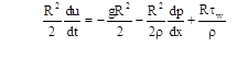
Multiplying the left and right sides of equation (2) by r, we write the individual terms of the equation of motion:

(3)

Where: friction; wall friction; dynamic viscosity; R is the radius of the cylindrical channel.

We use equations (3) and write equation (2) in the form (sloped brackets with an average speed are omitted hereinafter):



or

(four)

Let us choose in the cylindrical channel the volume of liquid by two cross sections at a distance . We write for the selected volume the balance of pressure and friction: , we obtain the ratio:

(five)

Using the Darcy-Weisbach equation combining it with (5) we get: , hence the ratio for friction of the liquid against the walls of the measuring channel will take the form:

(6)

where λ is the coefficient of hydraulic friction.

Substitute (6) into equation (4) and obtain the following expression:

(7)

Calculate the pressure gradient under the following conditions: the pressure decreases linearly from the boost pressure over the free surface of the fuel to the pressure . The pressure gradient with (1) will be equal to:

(eight)

Substituting (8) into the relation (7), we obtain the final differential equation for the level of liquid in the measuring channel:

(9)

With initial conditions of Cauchy, like:

(ten)

Solve the differential equation (9) with the initial conditions (10) [2].

Consider the conditions for measuring the level of liquid in the fuel tanks of the rocket in order to select the method of processing the measurement information using the solution of equation (9)

a) Level measurement in the absence of noise in the measuring channel and fuel oscillations. The dependence of the results of measuring the level of the flight time of the rocket is determined using the following program:

# -*- coding: utf8 -*- import numpy as np from scipy.integrate import odeint import matplotlib.pyplot as plt R=0.0195 #      H=8.2#     ,   g=9.8#     /2 L=4.83*10**-2#    V=0.039#       / def f(y,t): y1,y2=y return [y2,-g+(g*(HV*t)/y1)+((L/(4*R))*y2**2)] t = np.arange(0,10,0.01) y0=[H,0] [y1,y2]=odeint(f,y0,t,full_output=False).T plt.title('     ') plt.ylabel('H,m') plt.xlabel('t,s') plt.plot(t,y1,"b",linewidth=2,label='     ') y=HV*t plt.plot(t,y,"--r",linewidth=2,label='    ') plt.grid(True) plt.legend(loc='best') plt.show()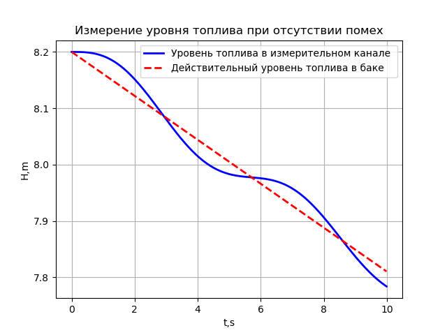 

This is an apparent solution to the first problem (due to graduation) when the level in the measuring channel lags behind the level in the tank. Since in real conditions of operation, fluctuations in the level and noise of the sensors introduce a significant error in the measurement.

b) Level measurement in the conditions of normally distributed random oscillations and noise with a dispersion of 0.1. The dependence of the results of measuring the level of the flight time of the rocket is determined using the following program:

 # -*- coding: utf8 -*- import numpy as np from scipy.integrate import odeint import matplotlib.pyplot as plt R=0.0195 #      H=8.2#     ,   g=9.8#     /2 L=4.83*10**-2#    V=0.039#       / def f(y,t): y1,y2=y return [y2,-g+(g*(HV*t)/y1)+((L/(4*R))*y2**2)] t = np.arange(0,10,0.01) y0=[H,0] [y1,y2]=odeint(f,y0,t,full_output=False).T y1= np.array([np.random.normal(x,0.1) for x in y1])#     plt.title('       \n      0.1') plt.ylabel('H,m') plt.xlabel('t,s') plt.plot(t,y1,"b",linewidth=2,label='     ') y=HV*t plt.plot(t,y,"--r",linewidth=2,label='    ') plt.grid(True) plt.legend(loc='best') plt.show()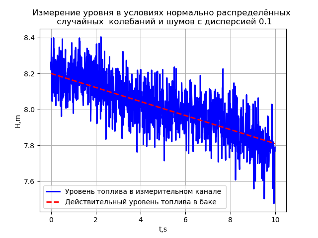 

The result confirms the conclusion that measuring the level in such conditions with an acceptable error of several percent of the range is impossible.

d) Level measurement under conditions of normally distributed random oscillations and noise with a dispersion of 0.1 using a Kalman filter. The dependence of the results of measuring the level of the flight time of the rocket is determined using the following program:

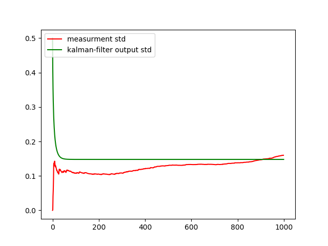
 # -*- coding: utf8 -*- from scipy.integrate import odeint import matplotlib.pyplot as plt from numpy import* from pykalman import KalmanFilter R=0.0195 H=8.2 g=9.8 L=4.83*10**-2 V=0.039 def f(y,t): y1,y2=y return [y2,-g+(g*(HV*t)/y1)+((L/(4*R))*y2**2)] t = arange(0,10,0.01) y0=[H,0] [y1,y2]=odeint(f,y0,t,full_output=False).T y=array(HV*t)#   measurements = array([random.normal(x,0.1) for x in y1]) kf = KalmanFilter(transition_matrices=[1] ,#  observation_matrices=[1],#  initial_state_mean=measurements[0],#   initial_state_covariance=1,#   observation_covariance=1,#  transition_covariance= 0.001) #   state_means, state_covariances = kf.filter(measurements)# ,   state_std = sqrt(state_covariances[:,0]) plt.figure() plt.title('      ') plt.ylabel('H,m') plt.xlabel('t,s') plt.plot(measurements, '-r', label='  ') plt.plot(state_means, '-g', label='kalman- ') plt.plot(y, '-k', label='  ') plt.legend(loc='best') plt.figure() measurement_std = [std(measurements[:i]) for i in arange(1,len(measurements),1)] plt.plot(measurement_std, '-r', label='measurment std') plt.plot(state_std, '-g', label='kalman-filter output std') plt.legend(loc='upper left') plt.show()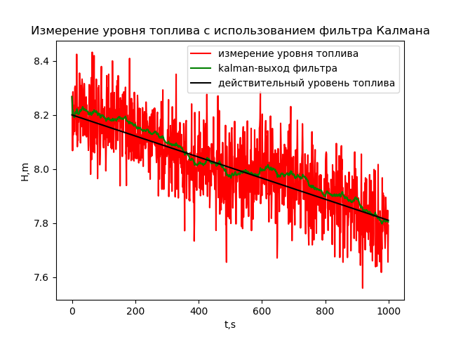 

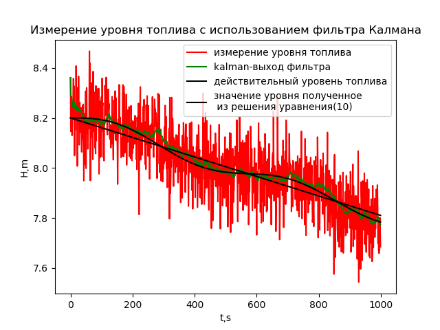
As can be seen from the graph, the filter eliminated random components and averaged values. However, the Kalman filter is “even smarter” and, with a certain setting, can even reduce the methodological error:

findings

Measuring the level of liquid in the fuel tanks of a rocket under conditions of normally distributed random fluctuations in the level and noise of sensors with a dispersion of 0.1 is possible only with the use of a Kalman filter.

Links

1. Measurement of the fluid level in the fuel tank of the rocket .
2. Suspended fuel tanks for aircraft .