Global lighting using voxel cone tracing
In this article I will talk about the implementation of one of the algorithms for calculating the global (re-reflected / ambient) lighting used in some games and other products - Voxel Cone Tracing (VCT). Perhaps someone read an old article ([VCT]) of 2011 or watched a video . But the article does not give exhaustive answers to the questions of how to implement a particular stage of the algorithm.
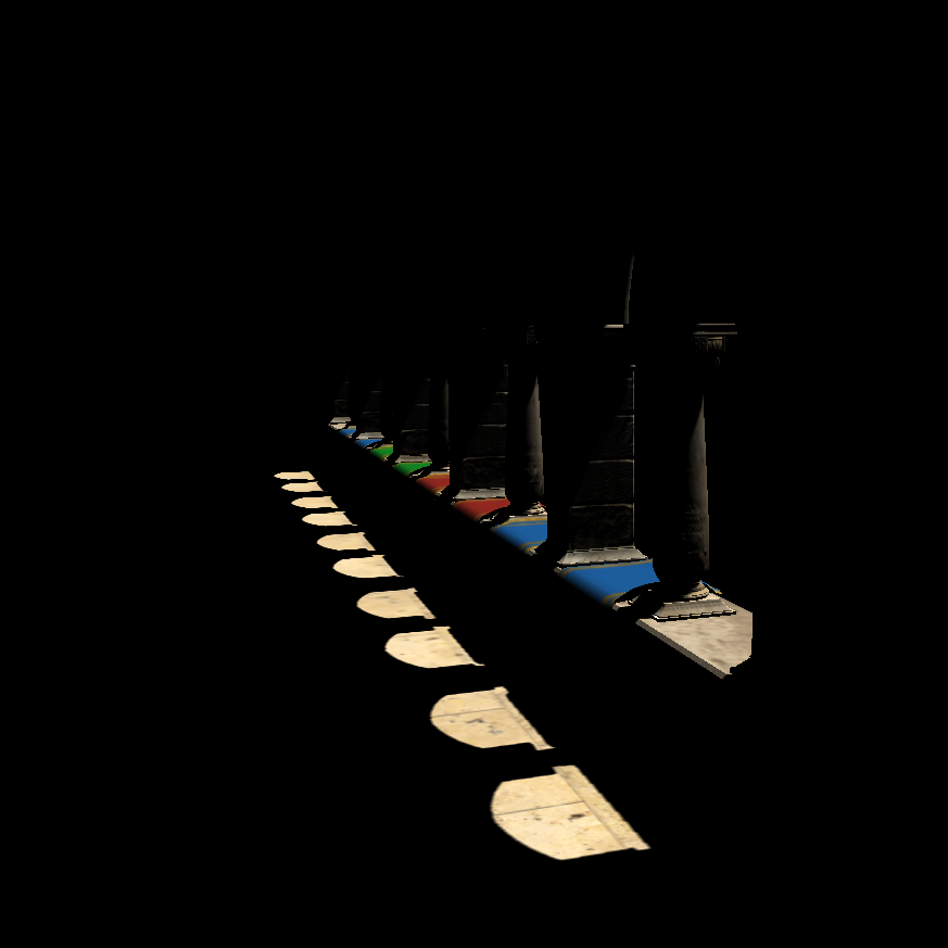
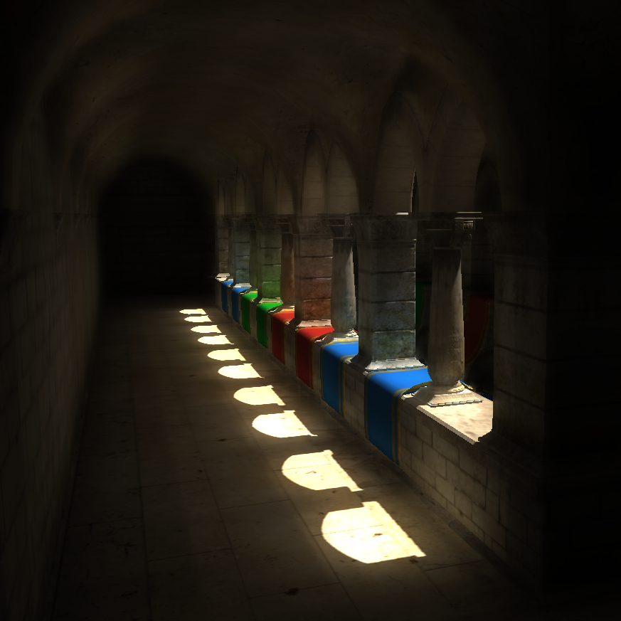
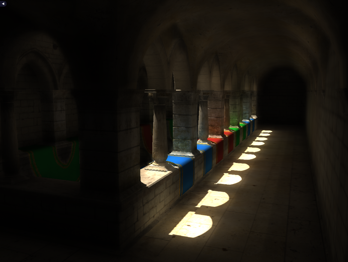
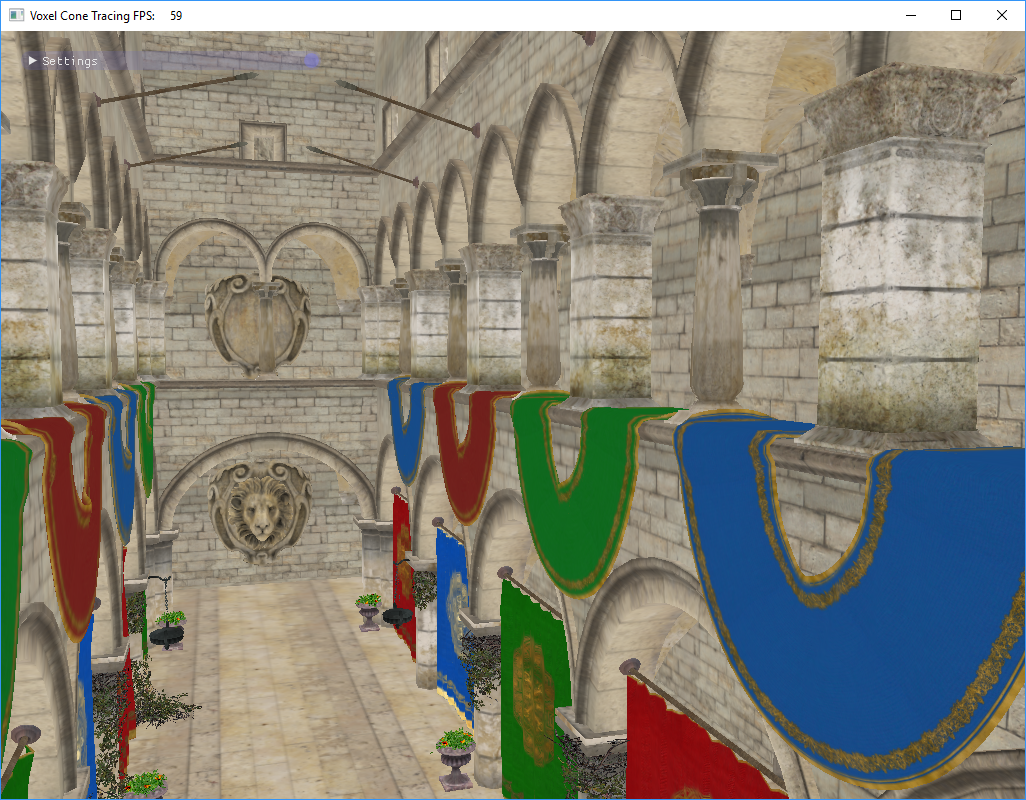
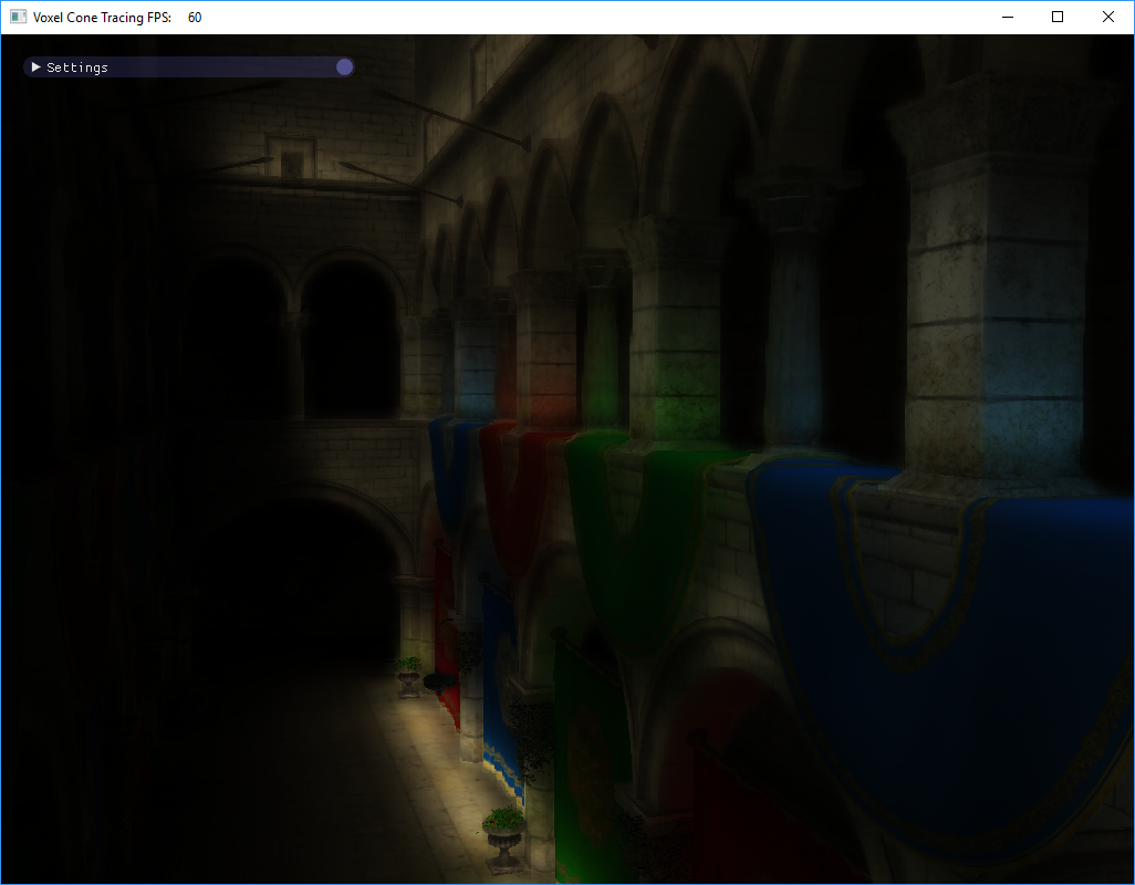
Render scenes without global illumination, and using VCT:
First of all, it is worth saying that the implementation of global illumination using environment maps (PMREM / IBL) is cheaper than VCT. For example, one of the developers of UE4 told in a podcast (1:34:05 - 1:37:50) that they rendered a demo using VCT, and then using environment maps, and the picture was about the same. However, research is being conducted under this approach. His ideas, for example, are based on Nvidia’s modern VXGI.
While working, I relied on a bunch of sources that can be found at the end of the article.
To simplify the task, the implementation takes into account only diffuse illumination (Labmert model), but it is argued that this algorithm is suitable for many other BRDF. Also, the implementation does not take into account the dynamic objects of the scene.
')
I will describe the implementation in terms of DirectX, but this algorithm can also be implemented on OpenGL. Some DX 11.1 chips are used in this work (for example, using a UAV in a vertex shader), but you can do without them, thereby lowering the minimum system requirements for this algorithm.
For a better understanding of the operation of the algorithm, we describe its general stages, and then we detail each of them. The most common parts of the algorithm are:
These stages can have several conceptual variants of implementations or contain additional optimizations. I want to show in a general form how this can be done.
To begin with, we will define the storage structure of the voxelized scene. You can voxelize all objects in a 3D texture. The disadvantage of this solution is non-optimal memory consumption, because most of the scene is empty space. For voxelization with a resolution of 256x256x256 of the format R8G8B8A8, this texture will take 64 MB, and this is without taking into account the MIPs. Such textures are required for color and normal surfaces, as well as for baked lighting.
Data optimization algorithms are used to optimize memory consumption. In our implementation, we will use Sparse Voxel Octree (SVO), as in the original article. But there are other algorithms, for example, 3D Clipmap [S4552].
SVO is a sparse octree scene. Each node of such a tree divides the scene's subspace into 8 equal parts. A sparse tree does not store information about a space that is not occupied by anything. We will use this structure to search for voxels by their coordinates in space, as well as to sample baked lighting. Baked lighting will be stored in a special 3D-texture - block buffer, which will be discussed below.
Consider each of the stages of the algorithm separately.
The voxelized scene will be stored as an array of voxels. On the GPU, this array is implemented through StructuredBuffer / RWStructuredBuffer. The voxel structure will be as follows:
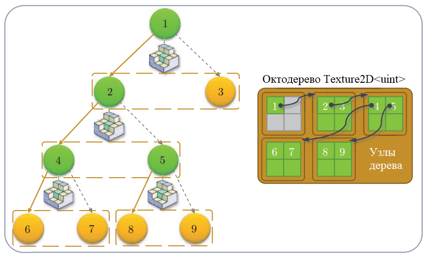
For compact scene storage, we use SVO. The tree will be stored in a 2D texture format R32_UINT. Tree node structure:

Schematic representation of the nodes SVO [DP]
In the leaves of SVO, the indices of the corresponding voxels from this array will be stored at the last level.
Suppose the resolution of our scene is 256x256x256, then to store a fully filled tree, we need a texture of 6185x6185 (145.9 MB). But we do not intend to store a full tree. According to my observations, for a Sponza scene with this resolution of the scene, a sparse tree is placed in a texture of 2080x2080 (16.6 MB).
To create an array of voxels, you need to voxelize all the objects in the scene. We use simple voxelization from the related article Octree-Based Sparse Voxelization . This technique is easy to implement and works in a single pass GPU.

Pipeline object voxelization [SV]
Calculate the bounding cube of the scene. Set the viewport by the resolution of the voxelized scene (for example, 256x256). We expose the orthographic camera above the stage to fit the bounding cube. Render every scene object we want to consider.
In a geometric shader, we handle the object's triangles. With the help of the normal of the triangle, the axis is chosen, in the direction of which the area of the projection of this triangle is maximal. Depending on the axis, we rotate the triangle with the largest projection to the rasterizer, so that we get more voxels.
In a pixel shader, each fragment will be a voxel. Create a Voxel structure with coordinates, color and normal, and add it to the voxel array.
At this stage, it is advisable to use low poly lody (LOD) objects in order not to have problems with missing voxels and merging voxels of adjacent triangles (such cases are discussed in article [SV]).

Voxelization artifacts - not all triangles are rasterized. Low poly lody should be used or additional triangles should be stretched.
When the whole scene is voxelized, we have an array of voxels with their coordinates. By this array, you can build SVO, with which we can find voxels in space. Initially, each pixel of the texture with SVO is initialized to 0xffffffff. To write tree nodes through a shader, the SVO texture will be represented as a UAV resource (RWTexture2D). To work with a tree, we will get an atomic node counter (D3D11_BUFFER_UAV_FLAG_COUNTER).
Let us describe in stages an octree creation algorithm. The node address in SVO is hereafter referred to as the node index, which is converted to 2D texture coordinates. By allocating a node we mean the following set of actions:
Schematic representation of the octree and its representation in texture [SV]
The algorithm for creating an octree with a height of N is as follows:
Having built such an octree tree, we can easily find the voxel of the scene by the coordinates in space, going down the SVO.
Now that we have designed the octree of the voxelized scene, we can use this information to preserve the illumination re-echoed by voxels from the light sources. Illumination is stored in a 3D texture format R8G8B8A8. This will allow us to use the trilinear interpolation of the GPU when sampling the texture, and as a result we will get a smoother final image. This texture is called the block buffer (brick buffer), because it consists of blocks arranged in accordance with SVO. A block is another representation of a group of voxels in space.
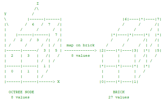
Groups of 2x2x2 voxels, whose indices are located in the leaves of the SVO, are mapped onto 3x3x3 voxels of 3D textures:
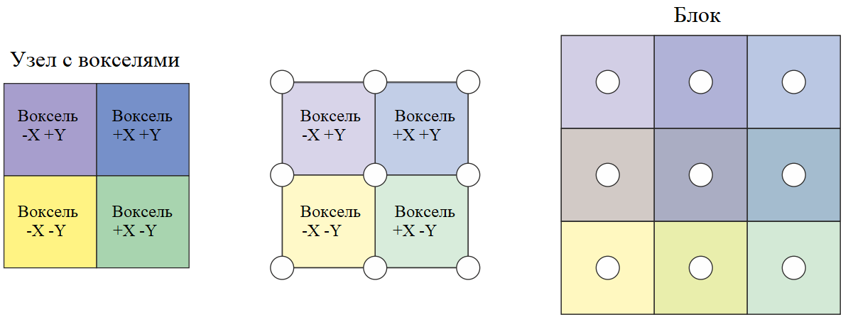
Display voxel group to voxel block [DP]
The voxel groups located in the scene next to each other may be scattered in the texture (since the texture is based on SVO). Therefore, for correct interpolation between adjacent groups of voxels, additional work is needed to average the values between adjacent blocks.

Averaging the boundaries of adjacent blocks
The voxels from the block are located at the corners of the original voxel group and between them. Thus, the blocks occupy more space in space than the original voxels. But sampling inside the block will be performed along the boundaries of the original voxels. So a semblance of a half-pixel-wide delimiter appears that is not used at all.
Blocks arranged according to the leaves of the SVO is a display of the original voxels. The blocks located in accordance with the remaining SVO nodes at certain octree levels are the MIP levels of the block buffer.

Schematic image of octree, its representation in texture and display in the buffer of blocks [SV]
The blocks do not have to be 3x3x3, they can be 2x2x2, and 5x5x5 - this is a question of the accuracy of the presentation. Blocks 2x2x2 would be another good way to save memory, but I have never met such an approach.

Interpolation comparison when sampling four adjacent voxels: without block buffer, from 3x3x3 block buffer and from 5x5x5 block buffer
Creating such a block buffer is quite time consuming. We will create two buffers: for storing scene transparency and for storing lighting.
The first step is to complete the voxels of the blocks matched with the leaves of the octree. Suppose we compute the reflected light in specific SVO voxels. Then these values will be mapped to the corresponding corner voxels of the block buffer.
After the calculation of the outgoing light is completed, for each block, we will fill in the remaining voxels with the averaged values of the neighboring voxels inside the block:
Now we average the values between adjacent blocks. That is why in the nodes of the tree neighbors are stored in space.

One of the options for averaging the block buffer is on each of the axes in three passes. Red rectangles indicate possible artifacts with this averaging [DP]
Create MIP levels of this buffer. The nodes of the upper levels of the SVO will be displayed in blocks that contain averaged values from the underlying level. Each block corresponding to a node from the top level of the tree includes information from the blocks of the corresponding descendants. It can also be blocks that correspond not only directly to the child nodes in the tree, but also to their neighbors (see the figure below).

On the left - the block includes information from the child blocks and their neighbors. Right - the block includes information only from child blocks [DP]
To reduce the number of memory accesses, for each calculated block, only voxels of child blocks are used (right figure). After that, the values between neighboring blocks are averaged, as described above. And so we create MIP levels until we reach the SVO root node.
Create two buffers - the scene transparency block buffer and the reflected light block buffer.
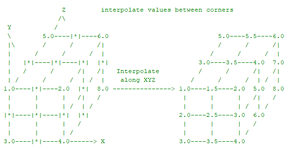
The transparency block buffer is created in advance, based on the voxelised geometry of the scene. We will keep the voxel directional transparency. To do this, fill in the RGB values of the voxels of the blocks from the lower level in accordance with the transparency of the voxels, and when creating the MIP levels of the blocks for each calculated voxel, we choose the averaged maximum transparency value along the XYZ axes and save them to the corresponding RGB texture values. Such a solution helps to take into account the obstruction of light in space in a certain direction.
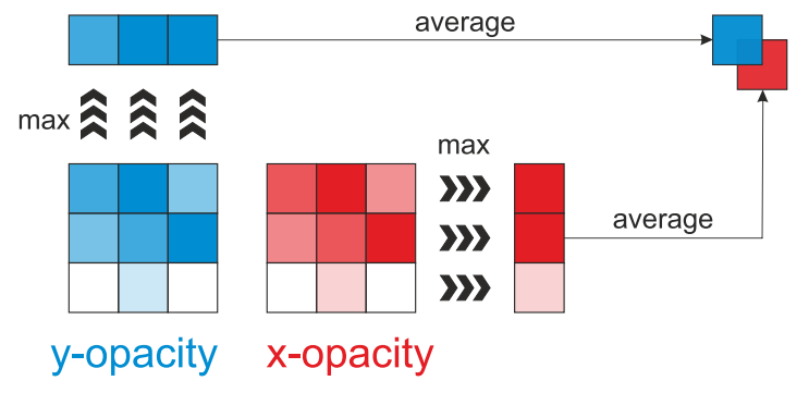
In each direction, a maximum is chosen in the value of transparency (that is, 1.0 is a completely opaque object, and this value will be maximum). Further, when constructing MIP levels, the maxima along the XYZ axes in the daughter blocks are averaged and added into the RGB components. [DP]
The illumination re-echoed by a voxel is calculated by processing the shadow map from the calculated light sources. Using this map, we can obtain the coordinates of objects in space and, using SVO, convert them into indices of illuminated voxels.
Normally, the shadow map resolution is higher than the octree resolution. The original article describes an approach in which each pixel of a shadow map is treated as a conditional photon. Accordingly, depending on the number of photons there will be a different contribution to the illumination. In my implementation, I simplified this stage and counted the illumination only once for each voxel that got into the shadow map.
To avoid recalculations, for each voxel for which reflected light has already been calculated, we use the flag bit of the octree node that stores the pointer to the voxel. Also, when processing a shadow map, among the pixels included in the same voxel, it is possible to select only the upper left for the calculation.


Fragment of the shadow map (left). On the right - in red, the top left pixels of the same voxel are shown.
Standard albedo * lightColor * dot (n, l) is used to calculate the reflected light, but in the general case it depends on BRDF. The calculated illuminance is written to the buffer of the lighting units. After processing the shadow map, the block buffer is refilled and MIP levels are created, as described above.
The algorithm is quite expensive. It is necessary to recalculate the buffer of the lighting units each time the lighting changes. One of the possible ways to optimize is to blur the update buffer by frame .
In order for a particular pixel to apply a trace of voxels by cones, you need to know the normal and the location of the pixel in space. These attributes are used to bypass the SVO and appropriately sample the lighting block buffer. You can get these attributes from G-buffer .
With G-buffer, it is also possible to calculate re-reflected lighting at a lower resolution than that of the viewport, which improves performance.
When the illumination block buffer is calculated, one can proceed to the calculation of the illumination re-reflected from the scene to the objects in the frame — that is, global illumination. For this, tracing voxels with cones is used.
For each pixel, several cones are emitted in accordance with BRDF. In the case of the Lambert lighting model, cones are emitted uniformly over a hemisphere oriented with the normal obtained from the G-buffer.

Emission of cones from the surface for which incoming lighting is calculated [VCT]
In the calculation, we assume that the illumination obtained from a point on the surface in the direction of the voxel will be the same as that emitted from the voxel towards the surface in a certain cone of visibility.
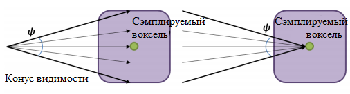
[VCT]
Tracing is done step by step. At each step, the illumination block buffer is sampled in accordance with the octree level (i.e., in accordance with the created MIP levels), starting with the lowest and ending at the highest.

Sampling the block buffer using a cone according to SVO levels [DP]
Taper tracing is done in the same way as volumetric objects [A] are rendered. Those. the alpha front-to-back model is used, in which at each next step along the cone, color and transparency are calculated as follows:
where a is transparency, c is the value obtained from the illumination block buffer multiplied by transparency (premultiplied alpha).
The transparency value is calculated using the transparency block buffer:
In other words, the transparency is read in the direction of the cone at a specific point. This is not the only approach. You can, for example, store transparency in the alpha channel of the illumination block buffer. But then the direction of re-reflected light is lost. I also tried to store directional illumination in six buffers of lighting units (two for each axis) - costs more than visible advantages.
The final result for the cones is weightedly summed up depending on the angles of the solution of the cones. If all the cones are the same, the weight is divided equally. The choice of the number of cones and the size of the angles of the solution is a matter of the ratio of speed and quality. In my implementation, there are 5 cones of 60 degrees (one in the center, and 4 on the sides).
The figure above shows schematically the sampling points along the axis of the cone. It is recommended to choose the location of the samples so that the octree node from the appropriate level fits into the cone. Or you can replace the corresponding sphere [SB]. But then sharp voxel borders may appear, so the location of the samples is adjusted. In my implementation, I just move the samples closer to each other.
As a bonus to re-reflected lighting, we also get Ambient Occlusion shading, which is calculated from the alpha value obtained by tracing. Also, when AO is miscalculated, at each step along the cone axis, a correction is made depending on the distance
The result is saved in an RGBA texture (RGB for lighting and A for AO). For a smoother result, a blur can be applied to the texture. The final result will depend on the BRDF. In my case, the calculated reflections are first multiplied by the surface albedo obtained from the G-buffer, then optionally multiplied by AO, and finally added to the main light.
In general, after certain settings and improvements, the picture is similar to the result from the article.


Comparison of the results - on the left is the scene rendered in Mental Ray, on the right is the Voxel Cone Tracing from the original article, in the center is my implementation.
The problem of self-illumination . Since in most cases the surface is physically located in its own voxels, it is necessary to somehow deal with self-illumination. One solution is to move the beginning of the cones in the direction of the normals. Also, this problem can theoretically be avoided if the directed distribution of light is stored in voxels.
Performance problem The algorithm is quite complicated, and you have to spend a lot of time on effective implementation on the GPU. I wrote the implementation "in the forehead", applying fairly obvious optimization, and the load turned out to be high. At the same time, even an optimized algorithm when searching for voxels in a tree will require a lot of SVO texture samples dependent on each other.
In my implementation, I emit 5 cones, sampling block buffers for the 4 penultimate octree levels of 256x256x256. According to the Intel GPA, the relative performance distribution is as follows:
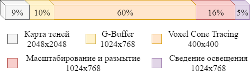
Performance Distribution G-Buffer and Shadow Map without pre-cool.
The original article uses three diffuse cones on a 512x512 texture on the whole SVO (512x512x512 - 9 levels). Together with direct lighting, it takes ~ 45% of the time frame 512x512. There is much to strive for. You also need to pay attention to optimizing the update buffer lighting.
Another problem with the algorithm is light leaking through objects . This happens with thin objects that make a small contribution to the transparency block buffer. Also, planes located near voxels of lower levels of SVO are subject to this phenomenon:

Light leaking: on the left - when using the VCT algorithm, on the right - in real life. This effect can be reduced with AO.
One more consequence follows from the above: it is not so easy to tweak the algorithm in order to get a good picture - how many cones to take, how many SVO levels, with which coefficients, etc.
We considered only static objects of the scene. To store dynamic objects, you need to modify the SVO and the corresponding buffers. As a rule, in this case, it is proposed to separately store static and dynamic nodes.
To summarize, I would not recommend this technique if you do not have enough time, patience and energy. But it will help to achieve a believable ambient lighting.
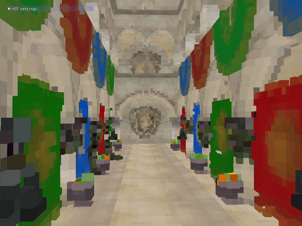
Dynamic demonstration:
Link to the application: https://github.com/Darkxiv/VoxelConeTracing (bin / VCT.exe)
The list of sources and resources that can help in the implementation of voxel tracing cones:
Render scenes without global illumination, and using VCT:
First of all, it is worth saying that the implementation of global illumination using environment maps (PMREM / IBL) is cheaper than VCT. For example, one of the developers of UE4 told in a podcast (1:34:05 - 1:37:50) that they rendered a demo using VCT, and then using environment maps, and the picture was about the same. However, research is being conducted under this approach. His ideas, for example, are based on Nvidia’s modern VXGI.
While working, I relied on a bunch of sources that can be found at the end of the article.
To simplify the task, the implementation takes into account only diffuse illumination (Labmert model), but it is argued that this algorithm is suitable for many other BRDF. Also, the implementation does not take into account the dynamic objects of the scene.
')
I will describe the implementation in terms of DirectX, but this algorithm can also be implemented on OpenGL. Some DX 11.1 chips are used in this work (for example, using a UAV in a vertex shader), but you can do without them, thereby lowering the minimum system requirements for this algorithm.
For a better understanding of the operation of the algorithm, we describe its general stages, and then we detail each of them. The most common parts of the algorithm are:
- Scene voxelization . We rasterize the scene into a set of voxels containing material properties (for example, color) and surface normals.

- Baking reflected lighting . For voxels, incoming or outgoing radiation from light sources is calculated, and the result is recorded in a 3D texture.


- Trace cones . For each calculated surface pixel, a group of cones is created. A cone is an abstraction that imitates a group of rays emitted to capture radiation from various mips of a 3D lighting texture. The end result is weighted averaged and stacked with the main light.

These stages can have several conceptual variants of implementations or contain additional optimizations. I want to show in a general form how this can be done.
To begin with, we will define the storage structure of the voxelized scene. You can voxelize all objects in a 3D texture. The disadvantage of this solution is non-optimal memory consumption, because most of the scene is empty space. For voxelization with a resolution of 256x256x256 of the format R8G8B8A8, this texture will take 64 MB, and this is without taking into account the MIPs. Such textures are required for color and normal surfaces, as well as for baked lighting.
Data optimization algorithms are used to optimize memory consumption. In our implementation, we will use Sparse Voxel Octree (SVO), as in the original article. But there are other algorithms, for example, 3D Clipmap [S4552].
SVO is a sparse octree scene. Each node of such a tree divides the scene's subspace into 8 equal parts. A sparse tree does not store information about a space that is not occupied by anything. We will use this structure to search for voxels by their coordinates in space, as well as to sample baked lighting. Baked lighting will be stored in a special 3D-texture - block buffer, which will be discussed below.
Consider each of the stages of the algorithm separately.
Voxelization scene
The voxelized scene will be stored as an array of voxels. On the GPU, this array is implemented through StructuredBuffer / RWStructuredBuffer. The voxel structure will be as follows:
struct Voxel { uint position; uint color; uint normal; uint pad; // 128 bits aligment }; For compact scene storage, we use SVO. The tree will be stored in a 2D texture format R32_UINT. Tree node structure:
Schematic representation of the nodes SVO [DP]
In the leaves of SVO, the indices of the corresponding voxels from this array will be stored at the last level.
Suppose the resolution of our scene is 256x256x256, then to store a fully filled tree, we need a texture of 6185x6185 (145.9 MB). But we do not intend to store a full tree. According to my observations, for a Sponza scene with this resolution of the scene, a sparse tree is placed in a texture of 2080x2080 (16.6 MB).
Create an array of voxels
To create an array of voxels, you need to voxelize all the objects in the scene. We use simple voxelization from the related article Octree-Based Sparse Voxelization . This technique is easy to implement and works in a single pass GPU.
Pipeline object voxelization [SV]
Calculate the bounding cube of the scene. Set the viewport by the resolution of the voxelized scene (for example, 256x256). We expose the orthographic camera above the stage to fit the bounding cube. Render every scene object we want to consider.
In a geometric shader, we handle the object's triangles. With the help of the normal of the triangle, the axis is chosen, in the direction of which the area of the projection of this triangle is maximal. Depending on the axis, we rotate the triangle with the largest projection to the rasterizer, so that we get more voxels.
In a pixel shader, each fragment will be a voxel. Create a Voxel structure with coordinates, color and normal, and add it to the voxel array.
At this stage, it is advisable to use low poly lody (LOD) objects in order not to have problems with missing voxels and merging voxels of adjacent triangles (such cases are discussed in article [SV]).
Voxelization artifacts - not all triangles are rasterized. Low poly lody should be used or additional triangles should be stretched.
Creating an octree using a voxel list
When the whole scene is voxelized, we have an array of voxels with their coordinates. By this array, you can build SVO, with which we can find voxels in space. Initially, each pixel of the texture with SVO is initialized to 0xffffffff. To write tree nodes through a shader, the SVO texture will be represented as a UAV resource (RWTexture2D). To work with a tree, we will get an atomic node counter (D3D11_BUFFER_UAV_FLAG_COUNTER).
Let us describe in stages an octree creation algorithm. The node address in SVO is hereafter referred to as the node index, which is converted to 2D texture coordinates. By allocating a node we mean the following set of actions:
- With the help of the current value of the node counter, addresses are calculated in which the child nodes of the node being located will be located.
- The node count is increased by the number of child nodes (8).
- Addresses of child nodes are written in the fields of the current node.
- In the flag field of the current node, it is written that it is allocated.
- The address of the current node is recorded in the parent field of the child nodes.
Schematic representation of the octree and its representation in texture [SV]
The algorithm for creating an octree with a height of N is as follows:
- Allocate the root node . The current tree level = 1. Node counter = 1.
- We touch the voxels . For each voxel, we find a node (subspace) at the current level of the tree to which it belongs. We mark such nodes with a flag that allocation is necessary. This stage can be parallelized on the vertex shader using Input-Assembler without buffers , using only the number of voxels and the SV_VertexID attribute for addressing over the array of voxels.
- For each node of the current tree level, check the flag . If necessary, allocate the node. This stage can also be parallelized on the vertex shader.
- For each node of the current tree level, we write in the child nodes of the neighbors' addresses .
- The current tree level is ++ . Repeat steps 2-5 until the current level of the tree is <N.
- At the last level, instead of allocating the current node, write the voxel index in the voxel array . Thus, the nodes of the last level will contain up to 8 indices.
Having built such an octree tree, we can easily find the voxel of the scene by the coordinates in space, going down the SVO.
Creating block buffer by octree tree
Now that we have designed the octree of the voxelized scene, we can use this information to preserve the illumination re-echoed by voxels from the light sources. Illumination is stored in a 3D texture format R8G8B8A8. This will allow us to use the trilinear interpolation of the GPU when sampling the texture, and as a result we will get a smoother final image. This texture is called the block buffer (brick buffer), because it consists of blocks arranged in accordance with SVO. A block is another representation of a group of voxels in space.
Groups of 2x2x2 voxels, whose indices are located in the leaves of the SVO, are mapped onto 3x3x3 voxels of 3D textures:
Display voxel group to voxel block [DP]
The voxel groups located in the scene next to each other may be scattered in the texture (since the texture is based on SVO). Therefore, for correct interpolation between adjacent groups of voxels, additional work is needed to average the values between adjacent blocks.
Averaging the boundaries of adjacent blocks
The voxels from the block are located at the corners of the original voxel group and between them. Thus, the blocks occupy more space in space than the original voxels. But sampling inside the block will be performed along the boundaries of the original voxels. So a semblance of a half-pixel-wide delimiter appears that is not used at all.
Blocks arranged according to the leaves of the SVO is a display of the original voxels. The blocks located in accordance with the remaining SVO nodes at certain octree levels are the MIP levels of the block buffer.
Schematic image of octree, its representation in texture and display in the buffer of blocks [SV]
The blocks do not have to be 3x3x3, they can be 2x2x2, and 5x5x5 - this is a question of the accuracy of the presentation. Blocks 2x2x2 would be another good way to save memory, but I have never met such an approach.
Interpolation comparison when sampling four adjacent voxels: without block buffer, from 3x3x3 block buffer and from 5x5x5 block buffer
Creating such a block buffer is quite time consuming. We will create two buffers: for storing scene transparency and for storing lighting.
Steps for creating a block buffer
The first step is to complete the voxels of the blocks matched with the leaves of the octree. Suppose we compute the reflected light in specific SVO voxels. Then these values will be mapped to the corresponding corner voxels of the block buffer.
After the calculation of the outgoing light is completed, for each block, we will fill in the remaining voxels with the averaged values of the neighboring voxels inside the block:
Now we average the values between adjacent blocks. That is why in the nodes of the tree neighbors are stored in space.
One of the options for averaging the block buffer is on each of the axes in three passes. Red rectangles indicate possible artifacts with this averaging [DP]
Create MIP levels of this buffer. The nodes of the upper levels of the SVO will be displayed in blocks that contain averaged values from the underlying level. Each block corresponding to a node from the top level of the tree includes information from the blocks of the corresponding descendants. It can also be blocks that correspond not only directly to the child nodes in the tree, but also to their neighbors (see the figure below).
On the left - the block includes information from the child blocks and their neighbors. Right - the block includes information only from child blocks [DP]
To reduce the number of memory accesses, for each calculated block, only voxels of child blocks are used (right figure). After that, the values between neighboring blocks are averaged, as described above. And so we create MIP levels until we reach the SVO root node.
Create two buffers - the scene transparency block buffer and the reflected light block buffer.
The transparency block buffer is created in advance, based on the voxelised geometry of the scene. We will keep the voxel directional transparency. To do this, fill in the RGB values of the voxels of the blocks from the lower level in accordance with the transparency of the voxels, and when creating the MIP levels of the blocks for each calculated voxel, we choose the averaged maximum transparency value along the XYZ axes and save them to the corresponding RGB texture values. Such a solution helps to take into account the obstruction of light in space in a certain direction.
In each direction, a maximum is chosen in the value of transparency (that is, 1.0 is a completely opaque object, and this value will be maximum). Further, when constructing MIP levels, the maxima along the XYZ axes in the daughter blocks are averaged and added into the RGB components. [DP]
Baking reflected lighting
The illumination re-echoed by a voxel is calculated by processing the shadow map from the calculated light sources. Using this map, we can obtain the coordinates of objects in space and, using SVO, convert them into indices of illuminated voxels.
Normally, the shadow map resolution is higher than the octree resolution. The original article describes an approach in which each pixel of a shadow map is treated as a conditional photon. Accordingly, depending on the number of photons there will be a different contribution to the illumination. In my implementation, I simplified this stage and counted the illumination only once for each voxel that got into the shadow map.
To avoid recalculations, for each voxel for which reflected light has already been calculated, we use the flag bit of the octree node that stores the pointer to the voxel. Also, when processing a shadow map, among the pixels included in the same voxel, it is possible to select only the upper left for the calculation.
Fragment of the shadow map (left). On the right - in red, the top left pixels of the same voxel are shown.
Standard albedo * lightColor * dot (n, l) is used to calculate the reflected light, but in the general case it depends on BRDF. The calculated illuminance is written to the buffer of the lighting units. After processing the shadow map, the block buffer is refilled and MIP levels are created, as described above.
The algorithm is quite expensive. It is necessary to recalculate the buffer of the lighting units each time the lighting changes. One of the possible ways to optimize is to blur the update buffer by frame .
Create G-Buffer
In order for a particular pixel to apply a trace of voxels by cones, you need to know the normal and the location of the pixel in space. These attributes are used to bypass the SVO and appropriately sample the lighting block buffer. You can get these attributes from G-buffer .
With G-buffer, it is also possible to calculate re-reflected lighting at a lower resolution than that of the viewport, which improves performance.
Trace voxel traces
When the illumination block buffer is calculated, one can proceed to the calculation of the illumination re-reflected from the scene to the objects in the frame — that is, global illumination. For this, tracing voxels with cones is used.
For each pixel, several cones are emitted in accordance with BRDF. In the case of the Lambert lighting model, cones are emitted uniformly over a hemisphere oriented with the normal obtained from the G-buffer.
Emission of cones from the surface for which incoming lighting is calculated [VCT]
In the calculation, we assume that the illumination obtained from a point on the surface in the direction of the voxel will be the same as that emitted from the voxel towards the surface in a certain cone of visibility.
[VCT]
Tracing is done step by step. At each step, the illumination block buffer is sampled in accordance with the octree level (i.e., in accordance with the created MIP levels), starting with the lowest and ending at the highest.
Sampling the block buffer using a cone according to SVO levels [DP]
Taper tracing is done in the same way as volumetric objects [A] are rendered. Those. the alpha front-to-back model is used, in which at each next step along the cone, color and transparency are calculated as follows:
' = ' + ( 1 — ' ) * ' = ' + ( 1 — ' ) * where a is transparency, c is the value obtained from the illumination block buffer multiplied by transparency (premultiplied alpha).
The transparency value is calculated using the transparency block buffer:
opacityXYZ = opacityBrickBuffer.Sample( linearSampler, brickSamplePos ).rgb; alpha = dot( abs( normalize( coneDir ) * opacityXYZ ), 1.0f.xxx ); In other words, the transparency is read in the direction of the cone at a specific point. This is not the only approach. You can, for example, store transparency in the alpha channel of the illumination block buffer. But then the direction of re-reflected light is lost. I also tried to store directional illumination in six buffers of lighting units (two for each axis) - costs more than visible advantages.
The final result for the cones is weightedly summed up depending on the angles of the solution of the cones. If all the cones are the same, the weight is divided equally. The choice of the number of cones and the size of the angles of the solution is a matter of the ratio of speed and quality. In my implementation, there are 5 cones of 60 degrees (one in the center, and 4 on the sides).
The figure above shows schematically the sampling points along the axis of the cone. It is recommended to choose the location of the samples so that the octree node from the appropriate level fits into the cone. Or you can replace the corresponding sphere [SB]. But then sharp voxel borders may appear, so the location of the samples is adjusted. In my implementation, I just move the samples closer to each other.
As a bonus to re-reflected lighting, we also get Ambient Occlusion shading, which is calculated from the alpha value obtained by tracing. Also, when AO is miscalculated, at each step along the cone axis, a correction is made depending on the distance
1 / (1 + lambda * distance) , where lambda is the calibration parameter.The result is saved in an RGBA texture (RGB for lighting and A for AO). For a smoother result, a blur can be applied to the texture. The final result will depend on the BRDF. In my case, the calculated reflections are first multiplied by the surface albedo obtained from the G-buffer, then optionally multiplied by AO, and finally added to the main light.
In general, after certain settings and improvements, the picture is similar to the result from the article.
Comparison of the results - on the left is the scene rendered in Mental Ray, on the right is the Voxel Cone Tracing from the original article, in the center is my implementation.
Underwater rocks
The problem of self-illumination . Since in most cases the surface is physically located in its own voxels, it is necessary to somehow deal with self-illumination. One solution is to move the beginning of the cones in the direction of the normals. Also, this problem can theoretically be avoided if the directed distribution of light is stored in voxels.
Performance problem The algorithm is quite complicated, and you have to spend a lot of time on effective implementation on the GPU. I wrote the implementation "in the forehead", applying fairly obvious optimization, and the load turned out to be high. At the same time, even an optimized algorithm when searching for voxels in a tree will require a lot of SVO texture samples dependent on each other.
In my implementation, I emit 5 cones, sampling block buffers for the 4 penultimate octree levels of 256x256x256. According to the Intel GPA, the relative performance distribution is as follows:
Performance Distribution G-Buffer and Shadow Map without pre-cool.
The original article uses three diffuse cones on a 512x512 texture on the whole SVO (512x512x512 - 9 levels). Together with direct lighting, it takes ~ 45% of the time frame 512x512. There is much to strive for. You also need to pay attention to optimizing the update buffer lighting.
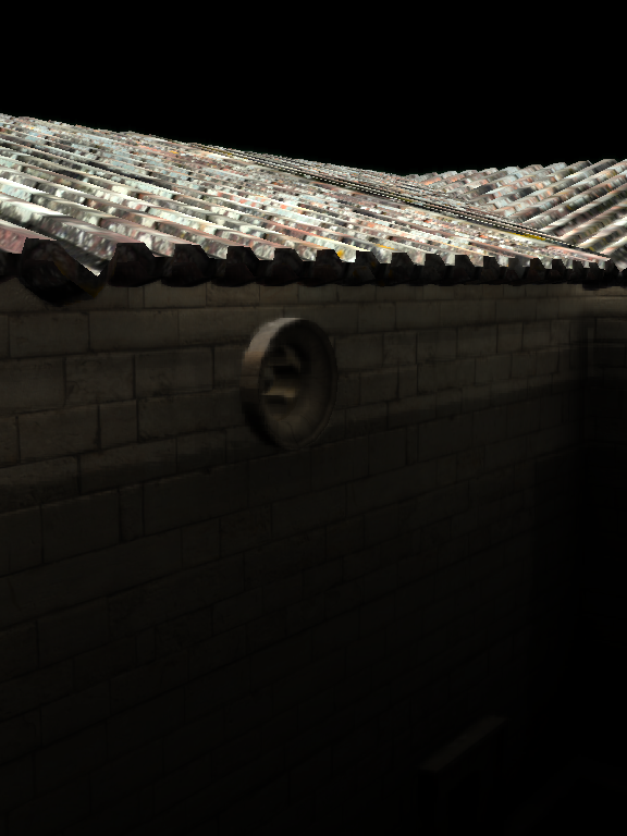
Another problem with the algorithm is light leaking through objects . This happens with thin objects that make a small contribution to the transparency block buffer. Also, planes located near voxels of lower levels of SVO are subject to this phenomenon:
Light leaking: on the left - when using the VCT algorithm, on the right - in real life. This effect can be reduced with AO.
One more consequence follows from the above: it is not so easy to tweak the algorithm in order to get a good picture - how many cones to take, how many SVO levels, with which coefficients, etc.
We considered only static objects of the scene. To store dynamic objects, you need to modify the SVO and the corresponding buffers. As a rule, in this case, it is proposed to separately store static and dynamic nodes.
To summarize, I would not recommend this technique if you do not have enough time, patience and energy. But it will help to achieve a believable ambient lighting.
Dynamic demonstration:
Link to the application: https://github.com/Darkxiv/VoxelConeTracing (bin / VCT.exe)
The list of sources and resources that can help in the implementation of voxel tracing cones:
- [VCT] Original article: http://research.nvidia.com/sites/default/files/publications/GIVoxels-pg2011-authors.pdf
- [SV] , SVO: https://www.seas.upenn.edu/~pcozzi/OpenGLInsights/OpenGLInsights-SparseVoxelization.pdf
- [S4552] NVIDIA: http://on-demand.gputechconf.com/gtc/2014/presentations/S4552-rt-voxel-based-global-illumination-gpus.pdf
- [A] alpha front-to-back: http://developer.download.nvidia.com/books/HTML/gpugems/gpugems_ch39.html
- [DP] , : http://dcgi.felk.cvut.cz/theses/2013/drinotom
- [SB] VCT: http://simonstechblog.blogspot.ru/2013/01/implementing-voxel-cone-tracing.html
- UE4: https://www.yumpu.com/en/document/view/4694219/the-technology-behind-the-elemental-demo-unreal-engine
- ambient : http://www.valvesoftware.com/publications/2006/SIGGRAPH06_Course_ShadingInValvesSourceEngine.pdf
- sparse octree NVIDIA https://developer.nvidia.com/gvdb
Source: https://habr.com/ru/post/353740/
All Articles