Associative rules, or beer with diapers

Introduction to theory

Education on association rules (hereinafter Associations rules learning - ARL) is, on the one hand, simple, on the other - quite often applicable in real life method of finding relationships (associations) in datasets, or, more precisely, data sets (itemsests). For the first time, Piatesky-Shapiro G [1] spoke in detail about this in “Discovery, Analysis, and Presentation of Strong Rules.” (1991) Agrawal R, Imielinski T, Swami A developed in more detail in “Mining Association Rules between Sets of Items in Large Databases ”(1993) [2] and“ Fast Algorithms for Mining Association Rules. ”(1994) [3] .

In general, ARL can be described as “Who bought x, also bought y”. It is based on the analysis of transactions, within each of which lies its own unique itemset from the set of items. With the help of the ARL aloglithms, there are those “rules” of the item matches within a single transaction, which are then sorted by their strength. Everything, in general, is simple.

Behind this simplicity, however, there can be hidden amazing things that common sense did not even suspect.
')
The classic case of such cognitive dissonance is described in the article DJ Power “Ask Dan!”, Published in DSSResources.com [4] .

In 1992, the Teradata retail consulting group led by Thomas Blyishok conducted a study of 1.2 million transactions in 25 stores for the Osco Drug retailer (no, they sold not drugs and not even drugs, or rather, not only drugs. Drug Store shops at home). After analyzing all these transactions, the strongest rule was “Between 17:00 and 19:00 most often beer and diapers buy together”. Unfortunately, such a rule seemed so counterintuitive to the leadership of Osco Drug that they did not put diapers on the shelves next to the beer. Although the explanation for the pair of beer-diapers was quite to be found: when both members of a young family were returning home from work (just at 5 o'clock in the evening), wives usually sent their husbands for diapers to the nearest store. And husbands, without hesitation, combined business with pleasure - they bought diapers on the instructions of the wife and beer for their own evening pastime.

Association rule description

So, we found out that beer and diapers are a good gentleman's set, and then what?
Suppose we have some dataset (or collection) D, such that $$$D = {d_0 ... d_j}$ where d is the unique transaction-itemset (for example, cash voucher). Each d is represented by a set of items (i - item) , and in the ideal case it is represented in binary form: d1 = [{Beer: 1}, {Water: 0}, {Coke: 1}, {...}], d2 = [{Beer: 0}, {Water: 1}, {Cola: 1}, {...}] . It is accepted that each itemset is described in terms of the number of nonzero values ​​( k-itemset ), for example, [{Beer: 1}, {Water: 0}, {Coke: 1}] is a 2-itemset .

If the dataset is not represented in binary form, you can convert it with your hands if you wish ( One Hot Encoding and pd.get_dummies can help you).

Thus, dataset is a sparse matrix with values ​​{1,0}. This will be a binary dataset. There are other types of record - vertical dataset (shows for each individual item a transaction vector, where it is present) and transactional dataset (approximately as in a cash voucher).

OK, the data is converted, how to find the rules?
There are a number of key (if you wish - basic) concepts in the ARL, which will help us derive these rules.

Support

The first concept in ARL is support:

$$

$$supp (X) = \ frac {\ {t \ in T; \ X \ in t \}} {| T |}$$

where X is an itemset containing i-items, and T is the number of transactions. Those. in general, it is an indicator of the “frequency” of a given itemset in all analyzed transactions. But this concerns only X. We are more interested in the option when we have x1 and x2 in one itemset (for example). Well, here too, everything is simple. Let x1 = {Beer}, and x2 = {Diapers} , then we need to count how many transactions this pair occurs.

$$

$$supp (x_1 \ cup x_2) = \ frac {\ sigma (x_1 \ cup x_2)} {| T |}$$

Where $$$\ sigma$ - number of transactions containing $$$x_1$ and $$$x_2$
Let's deal with this concept on a toy dataset.

play_set # microdataset, where transaction numbers are shown, and also presented in binary form what was bought on each transaction

$$

$$supp = \ frac {\ text {Transactions with beer and diapers}} {\ text {All transactions}} = P (\ text {Beer} \ cap \ text {Diapers})$$

$$

$$supp = \ frac {3} {5} = 60 \%$$

Confidence

The next key concept is confidence. This is an indicator of how often our rule works for the whole dataset.

$$

$$conf (x_1 \ cup x_2) = \ frac {supp (x_1 \ cup x_2)} {supp (x_1)}$$

Let's give an example: we want to count confidence for the rule “who buys beer, buys diapers”.

To do this, we first calculate what kind of support the “buy beer” rule has, then calculate the support of the rule “buy beer and diapers”, and simply divide one into the other. Those. we count in how many cases (transactions) the rule “bought beer” supp (X) works, “bought diapers and beer”

$$

$$supp (X \ cup Y)$$

Nothing like? Bayes looks at all this somewhat puzzled and with contempt.



Look at our microdataset.

$$

$$conf (\ text {Beer} \ cup \ text {Diapers}) = \ frac {supp (\ text {Beer} \ cup \ text {Diapers})} {supp (\ text {Beer})} = P (\ text {Diapers} \ mid \ text {Beer})$$

$$

$$conf = \ frac {3} {4} = 75 \%$$

Lift (support)

The next concept on our list is lift. Roughly speaking, lift is the relation of “dependency” items to their “independence”. Lift shows how items are dependent on each other. This is evident from the formula:

$$

$$lift (x_1 \ cup x_2) = \ frac {supp (x_1 \ cup x_2)} {supp (x_1) \ times supp (x_2)}$$

For example, we want to understand the dependence of the purchase of beer and the purchase of diapers. To do this, we consider the support rules “bought beer and diapers” and divide it by the product of the rules “bought beer” and “bought diapers”. In case lift = 1 , we say that items are independent and there are no joint purchase rules here. If lift> 1 , then the value by which lift, in fact, is greater than this very unit, and shows us the "power" of the rule. The larger the unit, the steeper. If lift <1, it will show that the base rule $ x_2 $ negatively affects the rule $ x_1 $. In another way, lift can be defined as the relation of confidence to expected confidence, i.e. the relationship of the credibility of the rule, when both (well, or whatever you want) elements are bought together to the reliability of the rule, when one of the elements was bought (whether with the second or not).

$$

$$lift = \ frac {\ text {Confidence}} {\ text {Expected confidence}} = \ frac {P (\ text {Diapers} \ mid \ text {Beer})} {P (\ text {Diapers})}$$

$$

$$lift = \ frac {\ frac {3} {4}} {\ frac {3} {5}} = $ 1.2$$

Those. our rule is that beer is bought with diapers, 25% more powerful than the rule that diapers just buy

Conviction

In general, Conviction is the “error rate” of our rule. That is, for example, how often they bought beer without diapers and vice versa.

$$

$$conv (x_1 \ cup x_2) = \ frac {1 - supp (x_2)} {1 - conf (x_1 \ cup x_2)}$$

$$

$$conv (\ text {Beer} \ cup \ text {Diapers}) = \ frac {1 - supp (\ text {Diapers})} {1 - conf (\ text {Beer} \ cup \ text {Diapers})} = \ frac {1 - 0.6} {1 - 0.75} = 1.6$$

The higher the formula 1, the better. For example, if conviction purchases of beer and diapers together would be equal to 1.2, this means that the rule “bought beer and diapers” would be 1.2 times (20%) more true than if the coincidence of these items in one transaction were pure random. A slightly non-intuitive concept, but it is not used as often as the previous three.

There are a number of commonly used classical algorithms that allow finding rules in itemsets according to the concepts listed above - the Naive or brute-force algorithm, the Apriori algorithm, the ECLAT algorithm, the FP-growth algorithm, and others.

Brutfors

Finding rules in itemsets is generally not difficult, difficult to do so effectively. Bruteforce algorithm is the easiest and, at the same time, the most inefficient way.

In pseudo-code, the algorithm looks like this:

INPUT : Dataset D, containing a list of transactions
OUTPUT : Sets itemsets $$$F_1, F_2, F_3, ... F_q,$ Where $$$F_i$ - a set of itemsets of size I, which occur at least s times in D
APPROACH :

1. R - integer array containing all combinations of items in D, size $$$2 ^ {| D |}$
2. for n $$$\ in$ [1, | D |] do:
F - all possible combinations of $$$D_n$
Increment each value in R according to the values ​​in each F []
3. return All itemsets in R $$$\ geq$ s

The complexity of the bruteforce algorithm is obvious:

In order to find all possible Association rules using a brute force algorithm, we need to list all the subsets X from set I and for each subset X calculate supp (X). This approach will consist of the following steps:

• generation of candidates . This step consists of enumerating all possible subsets of X subsets of I. These subsets are called candidates , since each subset can theoretically be a frequently encountered subset, then the set of potential candidates will consist of

  $$

  $$2 ^ {| D |}$$
  elements (here | D | denotes the number of elements of the set I, and

  $$

  $$2 ^ {| D |}$$
  often called the boolean of I, that is, the set of all subsets of I)
• calculation support . In this step, the supp (X) of each candidate X is calculated.

Thus, the complexity of our algorithm will be:

$$

$$O (| I | * | D | * 2 ^ {| I |})$$

where

$$

$$O (2 ^ {| I |})$$

- the number of possible candidates

$$

$$O (| I | * | D |)$$

- the complexity of the calculation of supp (X), since in order to calculate supp (X) we need to iterate over all the elements in I in each transaction

$$

$$t \ in T$$

In the O-large notation, we need O (N) operations, where N is the number of itemsets.
Thus, to apply the bruteforce algorithm, we need $$$2 ^ i$ memory cells, where i is an individual itemset. Those. for storage and calculation of 34 items we need 128GB of RAM (for 64-bit integer cells).

Thus, brute force will help us in the calculation of transactions in a tent with shawarma at the station, but for something more serious, it is completely unsuitable.

Apriori Algorithm

Theory

Used concepts:

• Many objects (itemset):

  $$

  $$X \ subseteq I = \ {x_1, x_2, ..., x_n \}$$
• Set of transaction identifiers (tidset):

  $$

  $$T = \ {t_1, t_2, ..., t_m \}$$
• Many transactions (transactions):

  $$

  $$\ {(t, \ X): \ t \ in T, \ X \ in I \}$$

Let us introduce some more concepts.

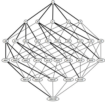
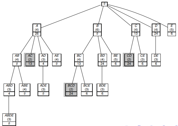
We will consider the prefix tree (prefix tree), where 2 elements X and Y are connected, if X is a direct subset of Y. Thus, we can enumerate all subsets of I. The figure is shown below:


So, consider the algorithm Apriori.

Apriori uses the following statement: if $$$X \ subseteq Y$ then $$$supp (X) \ geq supp (Y)$ .

The following 2 properties follow from here:

• if Y occurs often, then any subset

  $$

  $$X: X \ subseteq Y$$
  also common
• if X is rare, then any superset

  $$

  $$Y: Y \ supseteq X$$
  also rare

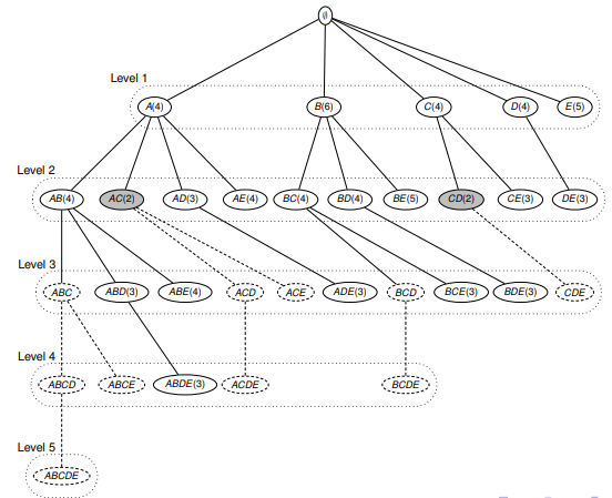
The Apriori algorithm, in a level manner, follows the prefix tree and calculates the frequency of occurrence of X subsets in D. Thus, in accordance with the algorithm:

• rare subsets and all their supersets are excluded
• calculate supp (X) for each suitable candidate X of size k at level k

In pseudo-code notation, the a priori algorithm looks like this:
INPUT : Dataset D, containing a list of transactions, and $$$\ sigma$ - user-defined threshold supp

OUTPUT : List itemsets F (D, $$$\ sigma$ )

APPROACH :

one. $$$C_1 \ leftarrow$ [{i} | i in J]
2. k $$$\ leftarrow$ one
3. while $$$C_k \ neq$ 1 do:
4. We consider all support for all candidates.
for all transactions (tid, I) $$$\ in$ D do:
for all candidates X $$$\ in$$$$C_k$ do:
if X $$$\ in$ I:
X.support ++
5. # Pull out all the frequent itemsets:
$$$F_k$ = {X | X.support> $$$\ sigma$ }
6. # Generating new candidates
$$$\ forall$ X, Y $$$\ in$$$$F_i$ , X [i] = Y [i] for 1 $$$\ leq$ i $$$\ leq$ k-1 and X [k] $$$\ leq$ Y [k] do:
I = x $$$\ cup$ {Y | k |}
if $$$\ forall$ J $$$\ subseteq$ I, | J | = k: J $$$\ in$$$$F_k$ then
$$$C_k + 1$$$$\ in$$$$C_k + 1$$$$\ cup$ I
k ++

Thus, Apriori first searches for all single (containing 1 element) itemsets that satisfy the user-defined supp, then makes pairs of them according to the principle of hierarchical monotony, i.e. if a $$$x_1$ is common and $$$x_2$ is common, then $$$[x_1, x_2]$ occurs often.

The obvious disadvantage of this approach is that it is necessary to “scan” the entire dataset, count all the supp at all levels. Breadth-first search ( search wide )
This can also bring up RAM on large datasets, although the algorithm in terms of speed is still much more efficient than bruteforce.

Implementation in python

from sklearn import ... ummm ... and there’s nothing to import. There are currently no modules for ALR in sklearn. Do not worry, google or write your own, right?

A variety of implementations are walking around the network, for example [here] , [here] , and even [here] .

In practice, we follow the apyori algorithm written by Yu Mochizuki. We will not give the full code, anyone can see [here] , but we will show the solution architecture and an example of use.

Conventionally, the solution Mochizuki can be divided into 4 parts: Data Structure, Internal Functions, API and Application Functions.

The first part of the module (Data Structure) works with the initial dataset. The TransactionManager class is implemented, whose methods combine transactions into a matrix, form a list of candidate rules, and consider support for each rule. In addition, internal functions, according to support, form lists of rules and rank them accordingly. The API logically allows you to work directly with datasets, and the Application functions allow you to process transactions and display the result in a readable form. No rocketscience.

Let's see how to use the module on a real (well, in this case, a toy) dataset.




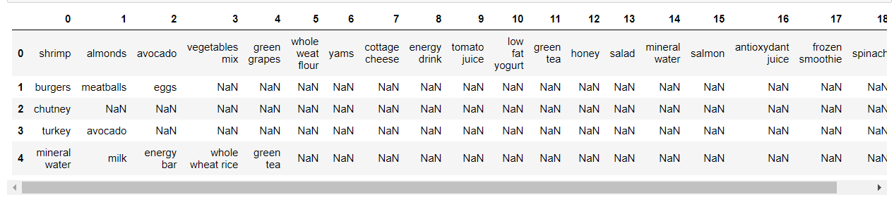
We see that our dataset represents a sparse matrix, where in rows we have a set of items in each transaction.

Replace NaN with the last value inside the transaction, so that later it would be easier to process the entire dataset.

 #    transactions = [] for i in range(0, 7501): transactions.append([str(dataset.values[i,j]) for j in range(0, 20)]) # apriori import apriori %%time #   .  ,          , #  ""     # min_support --  support   (dtype = float). # min_confidence --   confidence   (dtype = float) # min_lift --  lift (dtype = float) # max_length --   itemset (  k-itemset) (dtype = integer) result = list(apriori.apriori(transactions, min_support = 0.003, min_confidence = 0.2, min_lift = 4, min_length = 2)) 

Visualize the output




Total we see:

1. Pairs of items
2. items_base - the first element of the pair
3. items_add - the second (added by the algorithm) element of the pair
4. confidence - the value of confidence for a couple
5. lift - the lift value for the pair
6. support - the support value for the pair. If you wish, you can sort by

The results are logical: escalope and pasta, escalope and creamy mushroom sauce, chicken and low-fat sour cream, soft cheese and honey, etc. - all this is quite logical and, most importantly, delicious combinations.

Implementation in R

ARL is the case when R-Fils can giggle maliciously (java-Fils generally look at us mortals with contempt, but more on that below). In R, the arules library is implemented, where apriori and other algorithms are present. The official dock can be viewed [here]

Let's look at it in action:

First, install it (if not already installed).


We count the data and convert it into a transaction matrix.

Let's look at the data:

 summary(dataset) itemFrequencyPlot(dataset, topN = 10) 

The graph shows the frequency of individual items in transactions.



Let's learn our rules:

In general, the apriori call function looks like this:

 apriori(data, parameter = NULL, appearance = NULL, control = NULL) 

where

data - our dataset
parameter - the list of parameters for the model: minimum support, confidence and lift
appearance - responsible for displaying data. It can take values lhs, rhs, both, items, none , which determine the position of items in output
control - responsible for sorting the output (ascending, descending, without sorting), as well as whether to display the progress bar or not (the verbose parameter)

We will train model:

 rules = apriori(data = dataset, parameter = list(support = 0.004, confidence = 0.2)) 

And look at the results:

 inspect(sort(rules, by = 'lift')[1:10]) 

Make sure that the output has approximately the same results as when using the apyori module in Python:

1. {light cream} => {chicken} 0.004532729
2. {pasta} => {escalope} 0.005865885
3. {pasta} => {shrimp} 0.005065991
4. {eggs, ground beef} => {herb & pepper} 0.004132782
5. {whole wheat pasta} => {olive oil} 0.007998933
6. {herb & pepper, spaghetti} => {ground beef} 0.006399147
7. {herb & pepper, mineral water} => {ground beef} 0.006665778
8. {tomato sauce} => {ground beef} 0.005332622
9. {mushroom cream sauce} => {escalope} 0.005732569
10. {frozen vegetables, mineral water, spaghetti} => {ground beef} 0.004399413

ECLAT Algorithm

Theory

The idea of ​​the ECLAT (Equivalence CLAss Transformation) algorithm is to speed up the calculation of supp (X). To do this, we need to index our database D so that it allows us to quickly calculate supp (X)

It is easy to see that if t (X) denotes the set of all transactions where a subset of X occurs, then
t (XY) = t (X) $$$\ cup$ t (Y)
and
supp (XY) = | t (XY) |
that is, supp (XY) is equal to the cardinality (size) of the set t (XY)



This approach can be significantly improved by reducing the size of intermediate sets of transaction identifiers (tidsets). Namely, we can not store the entire set of transactions at the intermediate level, but only the many differences of these transactions. Let's pretend that

$$

$$X_a = \ {x_1, x_2, ..., x_ {n-1}, a \} X_b = \ {x_1, x_2, ..., x_ {n-1}, b \}$$

Then, we get:

$$

$$X_ {ab} = \ {x_1, x_2, ..., x_ {n-1}, a, b \}$$

$$$diffset (X_ {ab})$ this is the set of all transaction id that contains the X_a prefix, but does not contain the b element:

$$

$$d (X_ {ab}) = t (X_a) / t (X_ {ab}) = t (X_a) / t (X_ {b})$$

Unlike the Apriori algorithm, ECLAT searches in depth (DFS, [read more here] ). Sometimes referred to as “vertical” (as opposed to “horizontal” for Apriori)

INPUT : Dataset D, containing a list of transactions $$$\ sigma$ - user-defined threshold supp and new element prefix $$$I \ subseteq J$

OUTPUT : List itemsets F [I] (D, $$$\ sigma$ ) for the corresponding prefix I

AN APPROACH:
one. $$$F [i] \ leftarrow$ {}
2 $$$\ forall$ i $$$\ in$ J $$$\ in$ D do:
F [I]: = F [I] $$$\ in$ {I $$$\ in$ {i}}
3. Create $$$D_i$
$$$D_i \ leftarrow$ {}
$$$\ forall$ j $$$\ in$ J $$$\ in$ D $$$\ in$ j> i do:
C $$$\ cup$ ({i} $$$\ cup$ {j})
if | C | $$$\ geq \ sigma$ then
$$$D_i \ leftarrow D_i \ in {C, i}$
4. DFS - recursion:
Count $$$F | I | \ in {i} | (D_i, \ sigma)$
F [I]: F [I] $$$\ in$ F [I $$$\ in$ i]

The key concept for the ECLAT algorithm is the I-prefix. At the beginning, the empty set I is generated, this allows us to select all frequency itemsets on the first pass. Then the algorithm will call itself and increase I by 1 at each step until the user-specified length I is reached.

To store values, a prefix tree is used (trie (not tree :)), [more info here] . Initially, the zero root of the tree is built (that is the empty set I), then as it passes through the itemsets, the algorithm prescribes the contents of each itesmsets items, with the leftmost branch being the child of the zero root and further down. At the same time there are as many branches as items found in itemsets. This approach allows you to write an itemset in memory only once, which makes ECLAT faster than Apriori.

Implementation in python

There are several implementations of this algorithm in Python, those who wish can google and even try to get them to work, but we will write our own, as simple as possible and, most importantly, working.

 import numpy as np """   3 : - min_supp -  support     ItemSet.   %    - max_items -      ItemSet - min_items -    ItemSet """ class Eclat: #   def __init__(self, min_support = 0.01, max_items = 5, min_items = 2): self.min_support = min_support self.max_items = max_items self.min_items = min_items self.item_lst = list() self.item_len = 0 self.item_dict = dict() self.final_dict = dict() self.data_size = 0 #        ( ) def read_data(self, dataset): for index, row in dataset.iterrows(): row_wo_na = set(row[0]) for item in row_wo_na: item = item.strip() if item in self.item_dict: self.item_dict[item][0] += 1 else: self.item_dict.setdefault(item, []).append(1) self.item_dict[item].append(index) #   (instance variables) self.data_size = dataset.shape[0] self.item_lst = list(self.item_dict.keys()) self.item_len = len(self.item_lst) self.min_support = self.min_support * self.data_size #print ("min_supp", self.min_support) #     ItemSet   Eclat # : {Item: [Supp number, tid1, tid2, tid3, ...]} def recur_eclat(self, item_name, tids_array, minsupp, num_items, k_start): if tids_array[0] >= minsupp and num_items <= self.max_items: for k in range(k_start+1, self.item_len): if self.item_dict[self.item_lst[k]][0] >= minsupp: new_item = item_name + " | " + self.item_lst[k] new_tids = np.intersect1d(tids_array[1:], self.item_dict[self.item_lst[k]][1:]) new_tids_size = new_tids.size new_tids = np.insert(new_tids, 0, new_tids_size) if new_tids_size >= minsupp: if num_items >= self.min_items: self.final_dict.update({new_item: new_tids}) self.recur_eclat(new_item, new_tids, minsupp, num_items+1, k) #     def fit(self, dataset): i = 0 self.read_data(dataset) for w in self.item_lst: self.recur_eclat(w, self.item_dict[w], self.min_support, 2, i) i+=1 return self #    {ItemSet: support(ItemSet)} def transform(self): return {k: "{0:.4f}%".format((v[0]+0.0)/self.data_size*100) for k, v in self.final_dict.items()} 

We test on a toy sample:

 #       model = Eclat(min_support = 0.01, max_items = 4, min_items = 3) 

 # model.fit(dataset) 

 #   model.transform()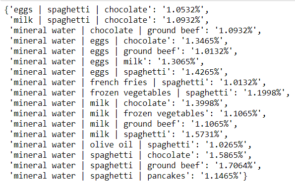 

Meanwhile in real-life ...

So, the algorithm works. But is it applicable in real life? Let's check.
There is a real business task that came to us from a large grocery retailer of the premium segment (we will not disclose the name and names of goods, corporate secrets): see the most frequent sets in grocery baskets.

Load the data from the unloading from the POS-system (Point-of-Sale - the system that processes transactions at the box office)




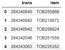
Change the table format to “transaction | list of all item in transaction




Run the algorithm

 model = Eclat(min_support = 0.0001, max_items = 4, min_items = 3) 

 %%time model.fit(df) 

Data read successfully
min_supp 9.755
CPU times: user 6h 47min 9s, sys: 22.2 s, total: 6h 47min 31s
Wall time: 6h 47min 28s

 model.transform()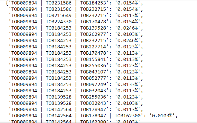 

On a regular computer, the solution to this puzzle took essentially a night. On cloud platforms it would be faster. But, most importantly, the customer is satisfied.

As you can see, implementing the algorithm on your own is quite simple, although it is worth working with efficiency.

Implementation in R
And again, users of R are jubilant, no dances with a tambourine are needed for them, all by analogy with apriori.

Run the library and read the data (to speed up, take the same toy dataset that apriori was counted on):


A quick look at dataset:

 summary(dataset) itemFrequencyPlot(dataset, topN = 10) 

Same frequencies as before



Rules:

 rules = eclat(data = dataset, parameter = list(support = 0.003, minlen = 2)) 

Note that we only configure support and the minimum length (k in k-itemset)

And look at the results:

 inspect(sort(rules, by = 'support')[1:10])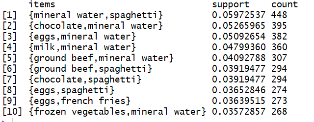 

FP-Growth Algorithm

Theory

The FP-Growth (Frequent Pattern Growth) algorithm is the youngest of our trinity, it was first described in 2000 in [7] .

FP-Growth offers a radical thing - to abandon the generation of candidates (recall, the generation of candidates is the basis of Apriori and ECLAT). Theoretically, such an approach would further increase the speed of the algorithm and use even less memory.

This is achieved by storing in memory a prefix tree (trie) not from combinations of candidates, but from the transactions themselves.

At the same time, FP-Growth generates a header table for each item, whose supp is higher than the one specified by the user. This header table stores a linked list of all similar nodes of the prefix tree. Thus, the algorithm combines the advantages of BFS at the expense of the header table and DFS by building trie. The pseudocode of the algorithm is similar to ECALT, with some exceptions.

INPUT : Dataset D, containing a list of transactions $$$\ sigma$ - user-defined threshold supp and prefix $$$I \ subseteq J$

OUTPUT : List itemsets F [I] (D, $$$\ sigma$ ) for the corresponding prefix I

APPROACH :

1. F [i] $$$\ leftarrow$ {}
2 $$$\ forall$ i $$$\ in$ J $$$\ in$ D do:
F [I]: = F [I] $$$\ in$ {I $$$\ in$ {i}}
3. Create $$$D_i$
$$$D_i \ leftarrow D_i$ {}
$$$H_i \ leftarrow$ {}
$$$\ forall$ j $$$\ in$ J $$$\ in$ D $$$\ in$ j> i do:
if supp (I $$$\ in$ {i, j}) $$$\ geq \ sigma$ then:
H $$$\ leftarrow$ H $$$\ in$ {j}
$$$\ forall$ (tid, X) $$$\ in$ D $$$\ subseteq$ I $$$\ in$ X do:
$$$D_i \ leftarrow D_i$$$$\ subseteq$ ({tid, X $$$\ in$ H})
4. DFS - recursion:
We consider F | I $$$\ in$ {i} | ( $$$D_i, \ sigma$ )
F [I] $$$\ leftarrow$ F [I] $$$\ subseteq$ F [I $$$\ subseteq$ i]

Implementation in python

Implementing FP-Growth in Python was no more lucky than other ALR algorithms. There are no standard libraries for it.

Not bad FP_Growth is presented in pyspark, watch [here]
On gitHub, you can also find several Neolithic solutions, for example [here] and [here]

Let's test the second option:

 #  patterns = pyfpgrowth.find_frequent_patterns(transactions, 2) #  rules = pyfpgrowth.generate_association_rules(patterns, 30); # rules 

Implementation in R

In this case, R is not far behind Python: there is no FP-Growth library in such a convenient and arules native library.

At the same time, as for Python, the implementation exists in Spark - [Link]

And in fact...

But in fact, if you want to use ARL in your business tasks, we strongly recommend learning Java .

Weka (Waikato Environment for Knowledge Analysis). This is a free Machine Learning Software written in Java. Worked out at the University of Waikato in New Zealand in 1993. Weka has both a GUI and the ability to work from the command line. The advantages include the ease of use of the graphical interface - there is no need to write code to solve applied problems. To use Weka libraries in Python, you can install a wrapper for Weka in Python: python-weka-wrapper3. The shell uses the javabridge package to access the Weka API. Detailed installation instructions can be found [here] .

SPMF This is an open source data mining library written in Java that specializes in searching patterns in data ( [link] ). It is stated that SPMF implemented more than 55 algorithms for mining data. Unfortunately, there is no official SPMF shell for Python (at least as of the date of this writing)

Conclusion or again about the effectiveness

In conclusion, let us compare empirically the effectiveness of the runtime metric depending on the density of the dataset and the length of the transaction dataset [9] .

Under the density dataset refers to the ratio of transactions, which contain frequent items to the total number of transactions.

Efficiency of algorithms at different densities



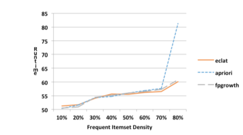
From the graph it is obvious that the efficiency (the lower the runtime, the more effective) the Apriori algorithm decreases with increasing density of the dataset.

Transaction length is the quantity in items in itemset

Efficiency of algorithms at different lengths



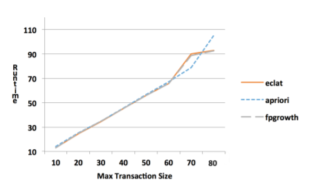
Obviously, by increasing the length of the transaction, Apriori also copes much worse.

To the question of the selection of hyperparameters

It's time to tell a little about how to choose the hyperparameters of our models (they are the very same support, confidence, etc.)

Since ARules algorithms are sensitive to hyperparameters, it is necessary to correctly approach the issue of choice. The difference in execution time for different combinations of hyperparameters may differ significantly.

The main hyper parameter in any ARules algorithm is min support. He, roughly speaking, is responsible for the minimum relative frequency of the associative rule in the sample. Choosing this indicator, you must first focus on the task. Most often, the customer needs a small number of top combinations, so you can set a high value of min support. However, in this case, some emissions may get into our sample ( bundle products , for example) and some interesting combinations may not be included. In general, the higher you set the caliper value, the more powerful the rules you find, and the faster the algorithm is considered. We recommend putting a smaller value on the first run to see which pairs, triples, etc. goods generally found in dataset. Then gradually increase the step, getting to the desired value (specified by the customer, for example). In practice, a good value of min supp will be 0.1% (with a very large dataset).

Below we provide an approximate graph of the dependence of the execution time of the algorithm on this indicator.



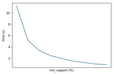
In general, everything as usual depends on the task and the data.

Results

So, we got acquainted with the basic theory of ARL ("who bought x, also bought y") and basic concepts and metrics (support, confidence, lift and conviction).

We looked at the 3 most popular (and old as the world) algorithms (Apriori, ECLAT, FP-Growth), envied the users of R and arules libraries, tried to implement ECLAT themselves.

Highlights:

1. ARL underlie recommendation systems
2. ARLs are widely applicable - from traditional retail and online retail (from Ozon to Steam), regular purchases of goods and materials to banks and telecom (connected services and services)
3. ARL is relatively easy to use, there are implementations of different levels of development for different tasks.
4. ARL are well interpreted and do not require special skills.
5. At the same time, algorithms, especially classical ones, cannot be called super-efficient. If you work with them out of the box on large datasets, you may need more processing power. But nothing prevents us from finishing them, right?

In addition to the considered basic algorithms, there are modifications and branches:

Algorithm CHARM for finding closed itemsets. This algorithm perfectly reduces the complexity of finding rules from exponential (that is, increasing with increasing dataset, for example) to polynomial. A closed itemset is an itemset for which there is no superset (i.e., a set that includes our itemset + other items) with the same frequency (= support).

Here it is worth explaining a little - until now we considered just frequent (frequent) itemsets. There is also the notion of closed (see above) and maximal ones . The maximum itemset is an itemset for which there is no frequent (= frequent) superset.

The relationship between these three types of itemsets is presented in the picture below:



AprioriDP (Dynamic Programming) - allows you to store supp in a special data structure, works slightly faster than the classic Apriori

FP Bonsai - improved FP-Growth with pruning a prefix tree (an example of an algorithm with constraints )

In conclusion, we cannot fail to mention the gloomy genius of ARL by Dr. Christian Borgelt from the University of Constance.

Christian implemented the algorithms we mentioned in C, Python, Java and R. Well, or almost everything. There is even a GUI for its authorship, where in a couple of clicks you can download datasets, select the desired algorithm and find the rules. This is provided that it will work for you.

For simple tasks, however, it is enough that we considered in this article. And if not enough, we urge you to write the implementation yourself!

References:

Discovery, analysis and presentation of strong rules. G. Piatetsky-Shapiro. Knowledge Discovery in Databases, AAAI Press, (1991)
Large Databases
Fast Algorithms for Mining Association Rules
Ask Dan!
Introduction to arules - A computational environment for mining
Publications by Dr. Borgelt
J. Han, J. Pei, and Y. Yin, “Mining session patterns,” in ACM SIGMOD Record, vol. 29, no. 2. ACM, 2000, pp. 1–12.
Shimon, Sh. Improving Data mining algorithms using constraints. The Open University of Israel, 2012.
Jeff Heaton. Fat-Growth Frequent Itemset Mining Algorithms
Sources

Authors: Pavel Golubev , Nikolay Bashlykov