Aircraft control system simulation

Hello!

In a previous article [1], we looked at some of the features of using the Python Control Systems Library for designing control systems. However, recently, the design of control systems using state variables has been widely used, which greatly simplifies the calculations.

Therefore, in this article, on the example of the control system from publication [2], we will consider a simplified model of autopilot using state variables and the tf, ss functions of the Control library.
')

Physical basis of the autopilot and the system of equations of flight

The equations governing the motion of an aircraft are a very complex set of six nonlinear coupled differential equations. However, under certain assumptions, they can be divided and linearized into the equations of longitudinal and lateral displacements. The flight of the aircraft is determined by the longitudinal dynamics.

Consider the work of the autopilot, which controls the height of the aircraft. The main axes and forces acting on the aircraft are shown in the figure below.



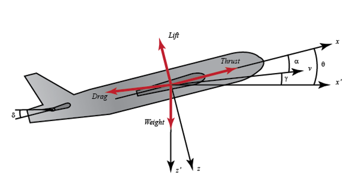
We assume that the aircraft is in stable flight with a constant height and speed, thus, the thrust, weight and lifting forces balance each other in the directions of the coordinate axes.

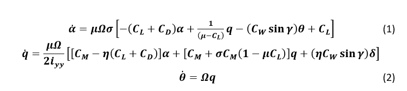
We also assume that changing the pitch angle will not under any circumstances change the flight speed (this is unrealistic, but it will slightly simplify the solution). Under these assumptions, the longitudinal equations of motion for an aircraft can be written as follows:



Designations of variables [3]:



For this system, the input will be the deflection angle and the output will be the pitch angle

Introduction of numerical values ​​to the equations of motion

Before finding the transfer functions from the space state model, let's include some numerical values ​​in order to simplify the above modeling equations:



These values ​​are taken from data from a commercial Boeing aircraft.

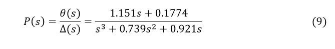
Transfer functions

To find the transfer function of this system, we need to take the Laplace transform from the above modeling equations. Recall that when finding the transfer function, zero initial conditions should be assumed. The Laplace transform of the above equations is shown below.



After a few steps of simple algebraic transformations, we must obtain the following transfer function:

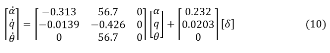
The state space of the control object

Recognizing the fact that the above modeling equations are already in the form of state variables, we can rewrite them as matrices, as shown below:



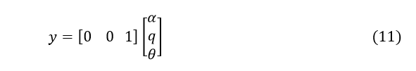
For the output characteristics of the model - the pitch angle, you can write the following equation:

The source data for the simulation

The next step is to select some design criteria. In this example, we develop a feedback controller, so that in response to the pitch pitch command, the actual pitch angle is less than 10%, the rise time is less than 2 seconds, the settling time is less than 10 seconds, and the steady error is less than 2%.

Thus, the source data requirements are as follows:

• Overload less than 10%
• Rise time less than 2 seconds
• Recovery time less than 10 seconds
• Stable error less than 2%

Python Tool Management System Simulation

Now we are ready to represent the system using Python. Below is a listing of the control system model in the state space.

from control import * num= [1.151, 0.1774] #    den= [1, 0.739, 0.921,0] #    P_pitch= tf(num, den) print("     (9):\n %s"%P_pitch) A = [[-0.313, 56.7, 0],[ -0.0139, -0.426, 0], [0, 56.7, 0]]; B = [[0.232], [0.0203],[0]]; C = [[0, 0, 1]]; D =[[0]]; pitch_ss = ss(A,B,C,D) print ("   \n     (10): \n \n %s"%pitch_ss) 

Result robots program:

Generation of transfer function by the relation (9):



The state space model of the control system according to equation (10):

A = [[-3.13e-01 5.67e + 01 0.00e + 00]
[-1.39e-02 -4.26e-01 0.00e + 00]
[0.00e + 00 5.67e + 01 0.00e + 00]]
B = [[0.232]
[0.0203]
[0. ]]
C = [[0 0 1]]
D = [[0]]

Conclusion: The Python Control Systems Library tools allow you to research control systems in the time domain using state variables.

References:

1. Using the Python Control Systems Library for designing automatic control systems.
2. Aircraft Pitch: System Modeling.
3. Extras: Aircraft Pitch System Variables.