In this article I will tell you how I managed to port the rendering algorithm of three-dimensional scenes to Excel formulas (without macros).

For those who are not familiar with computer graphics, I tried to describe all the steps as simply as possible and in more detail. In principle, for understanding the formulas should be enough knowledge of the school course of mathematics (+ the ability to multiply the three-dimensional matrix by the vector).
')
I also made a small web application where you can practice creating formulas for arbitrary shapes and generate your Excel file.

Caution: 19 pictures and 3 animations under the cut.

What happened

• File with cube and torus
• File with a kettle
• ObservableHQ laptop with its Excel files generator

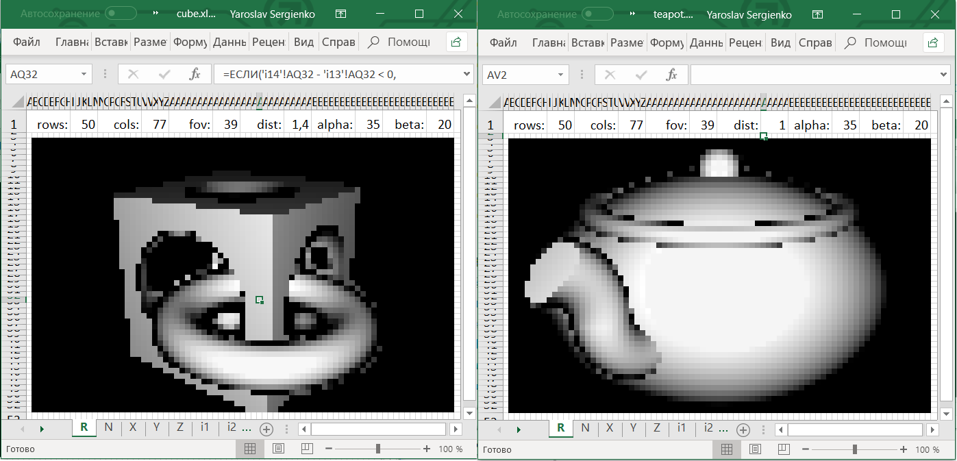
In Excel files at the top you can change the following cells:

• alpha: horizontal camera rotation in degrees
• beta: vertical camera rotation in degrees,
• dist: distance from the camera to the origin,
• fov: camera zoom.

To rotate the camera, you need to give Excel the right to change the file.

In the case of downloading your Excel file from ObservableHQ, the cells must be painted manually. You need to select all the small square cells and select “Conditional Formatting” → “Color Scales”.

Ray marching

The Ray Marching algorithm was popularized by Iñigo Quilez in 2008 after the presentation of Rendering Worlds with Two Triangles about a compact three-dimensional engine for the demostsen.

After that, Iñigo Quilez created the Shadertoy website, and most of the works sent there use the described methodology. It turned out that using it you can create photo-realistic scenes, see, for example, this gallery .

Ray Marching is a very easy-to-implement and efficient algorithm that allows rendering quite complex scenes. Why then is it not used on video cards? The fact is that video cards are sharpened to work with three-dimensional figures consisting of triangles, for which Ray Marching is not so effective.

Update: See also this comment from DrZlodberg about the disadvantages of this method.

The principle of the engine

• The object is described as a function.
• Match each pixel of the result of the beam leaving the camera.
• For each ray find the coordinates of the intersection with the object.
• At the intersection point to determine the color of the pixel.

I think that in one form or another, all these subtasks are solved in any three-dimensional engine.

Description of the object

You can think of three ways to describe a three-dimensional object:

• An explicit formula that, by a ray coming out of the camera, returns the point of intersection with the object (or, for example, the direction of the tangent in it).
• Membership function By a point in space, it tells whether it belongs to an object or not.
• Real function. For points inside the object, it is negative, outside - positive.

This article will use the special case of the third option, called the signed distance function (SDF) .

The SDF receives a point of space as input and returns the distance to the nearest point of the object. For points inside it is equal to the distance to the boundary of the object with a minus sign.

Finding the intersection of the beam and the object

Suppose we have a beam emanating from a camera, and we want to find its intersection point with an object.

Several ways come to mind to find this point:

• Go through the points on the ray with some steps.
• Having a point inside the object and outside, run a binary search to clarify the intersection.
• Either run any method for finding the roots of the SDF function (which is negative inside the object and positive outside) on the ray.

But here we will use another method: Ray Marching .

This is a simple algorithm that only works with SDF.



Let's parameterize the ray by distance from its beginning by the function $$$ray (t) = (x, y, z)$ .
Then $$$ray (0)$ - this is the camera itself. Here is the algorithm:

• $$$t = 0$
• To repeat $$$N$ time:
  
  • $$$t = t + SDF (ray (t))$
• If a $$$t <TMax$ then return $$$ray (t)$ as an intersection point, otherwise report that the ray does not intersect the object.

Here $$$N$ the number of iterations we can afford.
The more $$$N$ the more accurate the algorithm.

Number $$$TMax$ this is the distance from the camera, within which we expect to find the object.

Why does the algorithm work?

Does the algorithm always reach the point of intersection with the object (more precisely, it will strive for it)? The object may have a complex shape and its other parts may come close to the beam, preventing the algorithm from converging to the intersection point. In fact, this can not be: other parts of the object will necessarily be at some non-zero distance from the beam (otherwise it would intersect them), which we denote $$$\ delta> 0$ . Then the SDF function will be more $$$\ delta$ for any point of the ray (except for points very close to the intersection point). Therefore, sooner or later he will approach the point of intersection.


On the other hand, if the algorithm converges to a certain point, then the distance between adjacent iterations tends to zero. $$$\ Rightarrow$ SDF (distance to the nearest point of the object) also tends to zero $$$\ Rightarrow$ in the limit $$$Sdf = 0$$$$\ Rightarrow$ the algorithm converges to the point of intersection of the beam with the object.

Getting the color of the pixel at the intersection point

Imagine that for each pixel we found an intersection point with an object. We can draw these values ​​(that is, the distance from the camera to the point of intersection) directly and get these images:



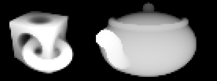
Given that this was obtained using Excel, not bad. But I want to know if it is impossible to make colors more similar to how we see objects in life.

In computer graphics, the basic method of calculating color is Phong shading . According to Phong, the resulting color consists of three components: background, specular and diffuse. Taking into account the fact that we are not striving for photo-realistic renders, it suffices to use only the diffuse component. The formula for this component follows from Lambert's law and states that the color of a pixel is proportional to the cosine of the angle between the normal to the surface and the direction to the light source.

Further, to simplify the calculations, assume that the light source and the camera are the same. Then we, in essence, need to find the sine of the angle between the beam emanating from the camera and the surface of the object:


Required angle $$$\ varphi$ I marked one arc in the drawing. The value of its sine is denoted as $$$k$ .

Usually, when using Ray Marching method, to find the normal to the object, do the following: consider the SDF value at six points (it is easy to reduce the number of points to four) near the intersection point and find the gradient of this function, which should coincide with the normal. It seemed to me that this is too much calculation for Excel, and I would like to find the desired angle easier.

If you look at the rate of convergence of the algorithm, you can see that if the angle between the ray and the object is straight, then one iteration is enough. If the angle is small, then the algorithm will converge very slowly.

Is it possible to get information about the angle to the surface based on the rate of convergence of the algorithm? If so, no additional calculations will be required at all: it is enough to analyze the values ​​of the previous iterations.

Draw a drawing. Denote $$$I_n$ and $$$I_ {n + 1}$ - points obtained at adjacent iterations of the algorithm. Suppose that the points are close enough to the object, that it can be replaced with a plane, the angle with which we want to find. Let be $$$R = SDF (I_n)$ , $$$r = SDF (I_ {n + 1})$ - distance from points $$$I_n$ and $$$I_ {n + 1}$ up the plane. Then, according to the algorithm, the distance between $$$I_n$ and $$$I_ {n + 1}$ equally $$$R$ .



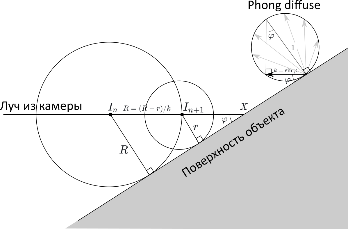
On the other hand, if we denote $$$X$ - the point of intersection of the ray and the figure, then
$$$I_nX = R / k$ , but $$$I_ {n + 1} X = r / k$ , Consequently

$$

$$R = I_nI_ {n + 1} = I_nX - I_ {n + 1} X = \ frac {R - r} {k}$$

$$

$$k = \ frac {R - r} {R} = 1 - \ frac {r} {R} = 1 - \ frac {SDF (I_ {n + 1})} {SDF (I_ {n})}$$

That is, the pixel intensity is equal to one minus the ratio of the SDF functions of adjacent iterations!

We describe simple shapes.

Examples of SDF for sphere, cube and torus:

$$$\ sqrt {x ^ 2 + y ^ 2 + z ^ 2} - r$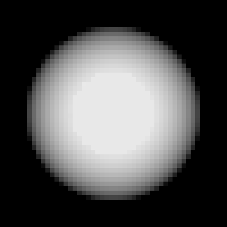
$$$\ max (| x |, | y |, | z |) - side / 2$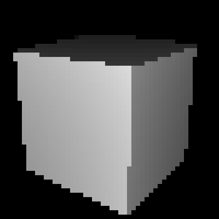
$$$\ sqrt {(\ sqrt {x ^ 2 + z ^ 2} - R) ^ 2 + y ^ 2} - r$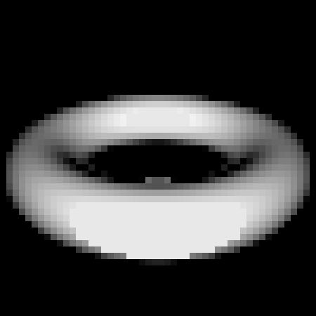

Shapes can be moved and compressed along the axes:

$$$cube (x, y + 0.3, z)$
$$$cube (x, 2 \ cdot y, z)$

Figures can also be combined, intersected and subtracted. That is, the SDF supports the basic operations of constructive solid geometry :

$$$\ min (sphere (x, y, z), cube (x, y, z))$
$$$\ max (sphere (x, y, z), cube (x, y, z))$
$$$\ max (-sphere (x, y, z), cube (x, y, z))$

The attentive reader may have noticed that in some figures (for example, a cube), as well as for some operations (for example, compression), the above formulas do not always return the distance to the nearest point of the object, that is, SDF is not formally. Nevertheless, it turned out that they can still be fed to the input of the SDF engine and it will correctly display them.

This is a small part of what you can do with the SDF, a full list of figures and operations can be found at www.iquilezles.org/www/articles/distfunctions/distfunctions.htm

Combining all the above formulas, we get the first figure:

$$$\ min (\\ \ quad \ max (| x | - 0.3, | y | - 0.3, | z | - 0.3, - \ sqrt {x ^ 2 + y ^ 2 + z ^ 2} + 0.375), \ \ \ quad \ sqrt {(\ sqrt {(x - 0.25) ^ 2 + (z - 0.25) ^ 2} - 0.25) ^ 2 + y ^ 2} - 0.05 \\)$

Formula Kettle

With a kettle a little harder: you need a plan



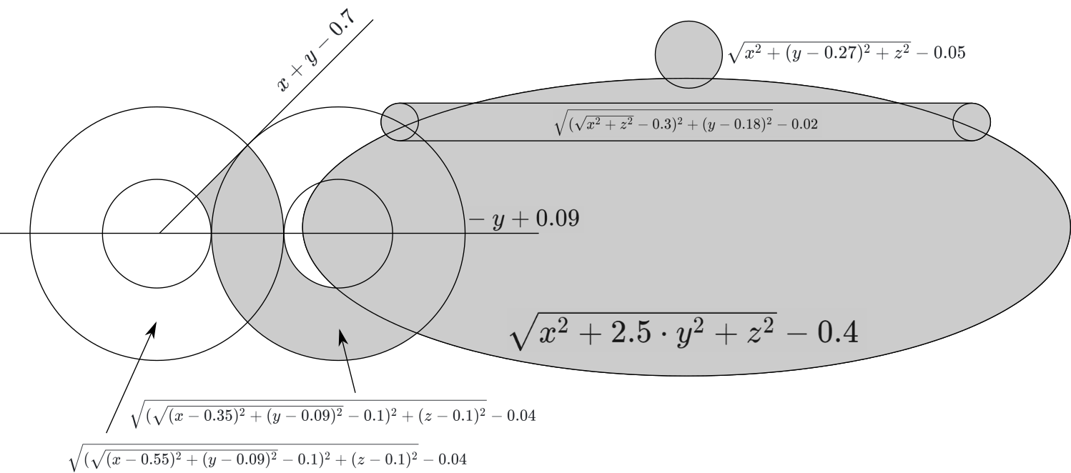
Carefully write the formula:

$$$\ min (\\ \ quad \ sqrt {x ^ 2 + (y - 0.27) ^ 2 + z ^ 2} - 0.05 \\ \ quad \ sqrt {x ^ 2 + 2.5 \ cdot y ^ 2 + z ^ 2 } - 0.4, \\ \ quad \ sqrt {(\ sqrt {x ^ 2 + z ^ 2} - 0.3) ^ 2 + (y - 0.18) ^ 2} - 0.02, \\ \ quad \ max (\\ \ qquad x + y - 0.7, \\ \ qquad - y + 0.09, \\ \ qquad \ sqrt {(\ sqrt {(x - 0.55) ^ 2 + (y - 0.09) ^ 2) - 0.1} ^ 2 + ( z - 0.1) ^ 2} - 0.04, \\ \ quad), \\ \ quad \ max (\\ \ qquad - (- y + 0.09), \\ qqad \ sqrt {(\ sqrt {(x - 0.35 ) ^ 2 + (y - 0.09) ^ 2} - 0.1) ^ 2 + (z - 0.1) ^ 2} - 0.04, \\ \ quad), \\)$

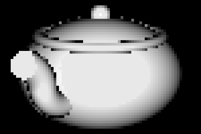
And we select the desired angle. Done:

---

Camera

All that is left for us is to find the corresponding beam in the space leaving the camera for a given pixel on the screen. More precisely, you must be able to find the point of this beam by distance from the camera. That is, we need a function $$$ray (s, t, d)$ where $$$s, t$ - pixel coordinates, and $$$d$ - distance from the beginning of the beam (camera).

For convenience of calculation, the coordinates of the pixels will be set relative to the center of the screen. Given that the screen consists of $$$rows$ rows and $$$cols$ columns, we expect coordinates within $$$s \ in \ left [- \ frac {cols} {2}, \ frac {cols} {2} \ right], t \ in \ left [- \ frac {rows} {2}, \ frac {rows} {2} \ right]$



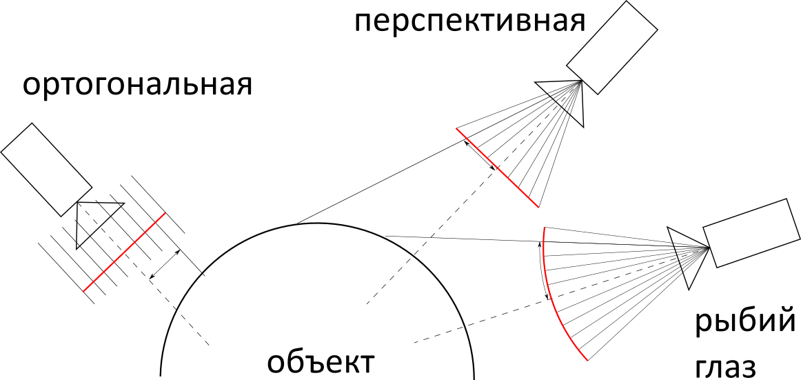
Next, you need to decide on the type of camera projection: orthogonal, perspective, or "fisheye." In terms of complexity of implementation, they are about the same, but in practice, perspective is most often used, so we will use it.



Most of the calculations in this chapter could have been avoided, for example, by placing the camera at a point $$$(1, 0, 0)$ and directing along the axis $$$X$ . But given the fact that the figures are also aligned along the axes, the result would not be a very interesting perspective. So in the case of a cube, we would see it as a square.

To ensure that the camera can be rotated, it is necessary to carefully conduct a number of calculations with Euler angles . So we get three input variables: angle $$$\ alpha$ angle $$$\ beta$ and distance $$$dist$ . They determine both the position and the direction of the camera (the camera always looks at the origin of coordinates).

With the help of WolframAlpha we find the rotation matrix:

$$

$$\ begin {pmatrix} x \\ y \\ z \ end {pmatrix} = \ underbrace {\ begin {pmatrix} \ cos (\ alpha) \ cos (\ beta) & - \ cos (\ alpha) \ sin ( \ beta) & \ sin (a) \\ \ sin (\ beta) & \ cos (\ beta) & 0 \\ - \ cos (\ beta) \ sin (\ alpha) & \ sin (\ alpha) \ sin (\ beta) & \ cos (\ alpha) \ end {pmatrix}} _ {M (\ alpha, \ beta)} \ begin {pmatrix} x '\\ y' \\ z '\ end {pmatrix}$$

If you apply it to a vector $$$(dist, 0, 0)$ , we will get the coordinates of the camera (do not ask me where the minus disappeared):

$$

$$\ begin {pmatrix} camX \\ camY \\ camZ \ end {pmatrix} = M (\ alpha, \ beta) \ begin {pmatrix} dist \\ 0 \\ 0 \ end {pmatrix} = dist \ begin {pmatrix } \ cos (\ alpha) \ cdot \ cos (\ beta) \\ \ sin (\ beta) \\ \ sin (\ alpha) \ cdot \ cos (\ beta) \ end {pmatrix}$$

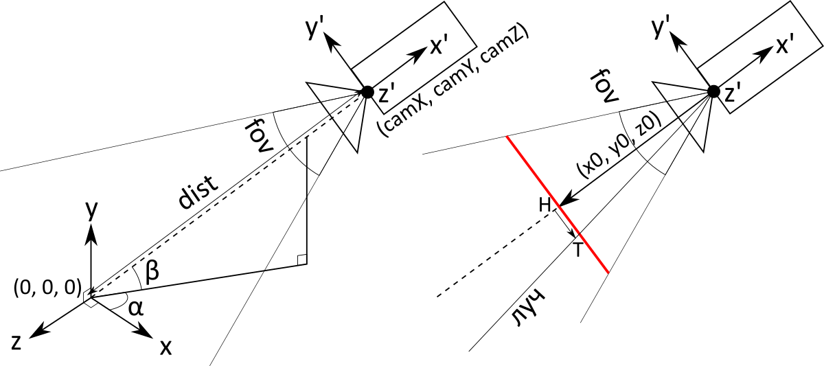
Subsequent calculations will be specific to the perspective projection. The main object is a screen (it is red in the figure, italic in the text). This is an imaginary rectangle at some distance in front of the camera, having, as you might guess, a one-to-one correspondence with the pixels of a regular screen. The camera is actually just a point with coordinates. $$$(camX, camY, camZ)$ . The rays corresponding to the pixels begin at the point of the camera and pass through the corresponding point on the screen .

The screen does not have exact location and size. More precisely, they depend on the distance to the camera: if you move the screen further, you will need to do more. Therefore, we agree that the distance from the camera to the screen is 1. Then we can calculate the value of the vector $$$(x0, y0, z0)$ connecting the point of the camera and the center of the screen (it is the same as at the center of the camera, only multiplied not by $$$dist$ and on $$$-1$ ):

$$

$$\ begin {pmatrix} x0 \\ y0 \\ z0 \ end {pmatrix} = M (\ alpha, \ beta) \ begin {pmatrix} -1 \\ 0 \\ 0 \ end {pmatrix} = - \ begin { pmatrix} \ cos (\ alpha) \ cdot \ cos (\ beta) \\ \ sin (\ beta) \\ \ sin (\ alpha) \ cdot \ cos (\ beta) \ end {pmatrix}$$

Now we need to determine the screen size. It depends on the angle of view of the camera, which is measured in degrees and corresponds to what is called “zoom” in video cameras. The user sets it with a variable. $$$fov$ (field of view). Since the screen is not square, it is necessary to clarify what is meant by the vertical viewing angle.

So, to determine the height of the screen, you need to find the base of an isosceles triangle with a vertex angle $$$fov$ and height 1: remembering trigonometry, we get $$$2 \ tan \ left (fov / 2 \ right)$ . Based on this, you can determine the size of one pixel on the screen :

$$

$$pixelSize = \ frac {2 \ tan \ left (fov / 2 \ right)} {rows}$$

Next, applying the rotation matrix to the vectors $$$(0, 0, 1)$ and $$$(0, 1, 0)$ get vectors $$$\ overline {u}$ and $$$\ overline {v}$ , setting the horizontal and vertical directions of the screen (to simplify the calculations, they are also pre-multiplied by $$$pixelSize$ ):

$$

$$\ begin {pmatrix} ux \\ uy \\ uz \ end {pmatrix} = pixelSize \ cdot M (\ alpha, \ beta) \ begin {pmatrix} 0 \\ 0 \\ 1 \ end {pmatrix} = pixelSize \ begin {pmatrix} \ sin (\ alpha) \\ 0 \\ \ cos (\ alpha) \ end {pmatrix}$$

$$

$$\ begin {pmatrix} vx \\ vy \\ vz \ end {pmatrix} = pixelSize \ cdot M (\ alpha, \ beta) \ begin {pmatrix} 0 \\ 1 \\ 0 \ end {pmatrix} = pixelSize \ begin {pmatrix} \ cos (\ alpha) \ cdot \ sin (\ beta) \\ \ cos (\ beta) \\ \ sin (\ alpha) \ cdot \ cos (\ beta) \ end {pmatrix}$$

Thus, we now have all the components to find the direction of the beam coming out of the camera and corresponding to the pixel with the coordinates $$$s, t$

$$

$$raydir (s, t) = \ begin {pmatrix} x0 \\ y0 \\ z0 \ end {pmatrix} + s \ begin {pmatrix} ux \\ uy \\ uz \ end {pmatrix} + t \ begin {pmatrix } vx \\ vy \\ vz \ end {pmatrix}$$

It is almost what you need. Only it is necessary to take into account that the beginning of the beam is at the point of the camera and that the direction vector must be normalized:

$$

$$ray (s, t, d) = \ begin {pmatrix} camX \\ camY \\ camZ \ end {pmatrix} + d \ cdot \ frac {raydir (s, t)} {\ lVert raydir (s, t) \ rVert}$$

So we got the desired function. $$$ray (s, t, d)$ which returns the point of the beam at a distance $$$d$ from its beginning, I correspond to a pixel with coordinates $$$s, t$ .

Excel

The Excel file that results is a book consisting of> 6 sheets:

• The first sheet of R contains everything the end user needs: the cells with parameters $$$rows, cols, fov, alpha, beta, dist$ , as well as cells with the result, painted on a black and white scale.
• Sheet N preassigns values $$$\ frac {1} {\ lVert raydir (s, t) \ rVert}$ .
• Sheets X , Y , Z calculate coordinates $$$X, y, z$ vectors $$$raydir (s, t)$ and $$$\ frac {raydir (s, t)} {\ lVert raydir (s, t) \ rVert}$ .
• Sheets i1 , i2 , ... contain iterations of the Ray Marching algorithm for each pixel.

All sheets are built according to the same scheme:

• The first line contains 1-6 “global” variables (blue). They can be used in all sheets.
• Most of the sheet is occupied by pixel calculations (green). This is a rectangle of size. $$$rows \ times cols$ . In the tables at the end of the article, these cells are designated as **
• Sheets X , Y, and Z also use intermediate calculations in rows and columns (orange). The second row and first column are reserved for them. In the tables at the end of the article, these cells are designated A* and *2 . The idea is that to store values $$$raydir (s, t)$ over all pixels it is not necessary to add three more sheets (for each of the coordinates) since the formula for its calculation is divided into the sum of two components:
  

  $$

  $$raydir (s, t) = \ underbrace {\ begin {pmatrix} x0 \\ y0 \\ z0 \ end {pmatrix} + s \ begin {pmatrix} ux \\ uy \\ uz \ end {pmatrix}} _ { \ mbox {by columns}} + \ underbrace {t \ begin {pmatrix} vx \\ vy \\ vz \ end {pmatrix}} _ {\ mbox {by rows}}$$
  
  Thus, we predict the first addendum by column and second by row, and when we need to get the value $$$raydir (s, t)$ we add the cell value to the row $$$s$ and column $$$t$ .
  

Sheet R
I1	rows:	50
V1	cols:	77
AI1	fov:	39
AV1	dist:	1,4
BI1	alpha:	35
Bv1	beta:	20
**	=(i14! XN - i13! XN < 0,00000000000001; 0,09; (0; (1; (i15! XN - i14! XN ) / (i14! XN - i13! XN ))))

Sheet N
I1	pixelSize:	=TAN(R!AI1 / 2) / (R!I1 / 2)
**	=1 / ((X!A N + X! X 2; 2) + (Y!A N ; 2) + (Z!A N + Z! X 2; 2))

Sheet X
I1	camX:	=R!AV1 * COS(R!BV1) * COS(R!BI1)
V1	ux:	=-N!I1 * SIN(R!BI1)
AI1	vx:	=N!I1 * SIN(R!BV1) * COS(R!BI1)
AV1	x0:	=-COS(R!BV1) * COS(R!BI1)
A *	=AI1 * (() - 2 - (R!I1 + 1) / 2)
* 2	=AV1 + V1 * (() - 1 - (R!V1 + 1) / 2)
**	=( Z 2 + A N ) * N! Z N

Sheet Y
I1	camY:	=R!AV1 * SIN(R!BV1)
V1	vy:	=-N!I1 * COS(R!BV1)
AI1	y0:	=-SIN(R!BV1)
A *	=AI1 + V1 * (() - 2 - (R!I1 + 1) / 2)
**	=A N * N! Z N

Sheet Z
I1	camZ:	=R!AV1 * COS(R!BV1)) * SIN(R!BI1)
V1	uz:	= N!I1 * COS(R!BI1)
AI1	vz:	= N!I1 * SIN(R!BV1) * SIN(R!BI1)
AV1	z0:	=-COS(R!BV1) * SIN(R!BI1)
A *	=AI1 * (() - 2 - (R!I1 + 1) / 2)
* 2	=AV1 + V1 * (() - 1 - (R!V1 + 1) / 2)
**	=( Z 2 + A N ) * N! Z N

I1 sheet
I1	dist0:	= formula( X!I1, Y!I1, Z!I1 )
**	=I1 + formula( X!I1 + X! XN * I1, Y!I1 + Y! XN * I1, Z!I1 + Z! XN * I1 )

Sheets i2 , i3 , ...
**	=i (n-1) ! XN + formula( X!I1 + X! XN * i (n-1) ! XN , Y!I1 + Y! XN * i (n-1) ! XN , Z!I1 + Z! XN * i (n-1) ! XN )

Notes:

• Since in Excel calculations are made in radians, the arguments of all trigonometric functions are multiplied by $$$\ frac {\ pi} {180}$ (Excel has a RADIANS function for this). In order not to confuse the formulas, I removed these multiplications in the tables above.
• Where the formula is written, you must insert one of these formulas:
  
  
  Excel cube formula

   MIN (
     MAX (
       ABS (x) - 0.3, ABS (y) - 0.3, ABS (z) - 0.3,
       -SQRT (POWER (x, 2) + POWER (y, 2) + POWER (z, 2)) + 0.375
     ),
     SQRT (POWER (SQRT (POWER (x - 0.25, 2) + POWER (z - 0.25, 2)) - 0.25, 2) + POWER (y, 2)) - 0.05
   )
  

  
  
  
  
  Excel Formula Teapot

   MIN (
     SQRT (POWER (SQRT (POWER (x, 2) + POWER (z, 2)) - 0.3, 2) + POWER (y - 0.18, 2)) - 0.02,
     SQRT (POWER (x, 2) + POWER (y, 2) * 2.5 + POWER (z, 2)) - 0.4,
     MAX (
       x + y - 0.15 - 0.05 - 0.5,
       - (y) + 0.19 - 0.1,
       SQRT (POWER (SQRT (POWER (x - 0.55, 2) + POWER (y - 0.09, 2)) - 0.1, 2) + POWER (z - 0.1, 2)) - 0.04
     ),
     MAX (
       - (- (y) + 0.19 - 0.1),
       SQRT (POWER (SQRT (POWER (x - 0.35, 2) + POWER (y - 0.09, 2)) - 0.1, 2) + POWER (z - 0.1, 2)) - 0.04
     ),
     SQRT (POWER (x, 2) + POWER (y - 0.27, 2) + POWER (z, 2)) - 0.05
   )
  

  
  
  
  

How does this article compare with the article “3D-engine written on MS Excel formulas” ?

That engine is only suitable for rendering mazes and ellipsoids. One-dimensional Raycaster is used, from which data stripes are created up and down creating the illusion of walls. But there is implemented a full-fledged game logic, here the goal is only a three-dimensional engine.