State space in problems of designing optimal control systems

Introduction

The study of the control system in the time domain using state variables has been widely used recently due to the simplicity of the analysis.

The state of the system corresponds to a point in a certain Euclidean space, and the system behavior in time is characterized by the trajectory described by this point.

At the same time, the mathematical apparatus includes ready-made solutions for analog and discrete LQR and DLQR controllers, Kalman filter, and all this with the use of matrices and vectors, which allows you to write the equations of the control system in a generalized form, obtaining additional information when solving them.
')
The purpose of this publication is to consider solving the problems of designing optimal control systems using the state space description method using Python software.

Theory briefly

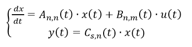
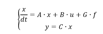
A vector-matrix record of a linear dynamic object model taking into account the measurement equation takes the form:

(one)

If the matrices A (t), B (t) and C (t) do not depend on time, then the object is called an object with constant coefficients, or a stationary object. Otherwise, the object will be non-stationary.

In the presence of errors in measurement, the output (adjustable) signals are given by the linearized matrix equation:

(2)

where y (t) is the vector of regulated (measured) values; C (t) is the coupling matrix of the measurement vector with the state vector; v (t) is the vector of measurement errors (interference).

The structure of a linear continuous system that implements equations (1) and (2) is shown in the figure:



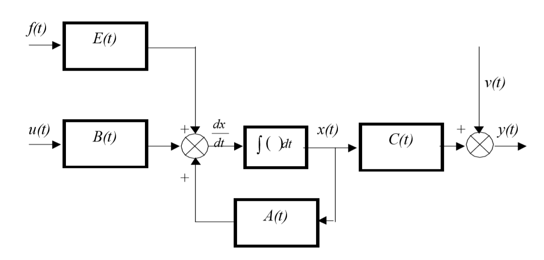
This structure corresponds to a mathematical model of an object constructed in the state space of its input x (t), u (t), output y (t), and internal, or phase coordinates x (t).

For example, consider the mathematical model of a DC motor with independent excitation from permanent magnets. The system of equations of the electric and mechanical parts of the engine for the case in question will look like this:

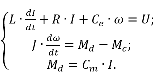(3)

The first equation reflects the relationship between the variables in the anchor chain, the second the mechanical equilibrium conditions. As the generalized coordinates, we choose the armature current I and the armature rotation frequency ω .

The control is the voltage at the anchor U , the disturbance is the moment of resistance of the load Mc . The parameters of the model are the resistance and inductance of the circuit and anchor, denoted respectively by R , and L , as well as the reduced moment of inertia J and the design constants ce and cm (in the SI system: Ce = cm ).

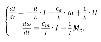
Solving the original system with respect to the first derivatives, we obtain the equations of the engine in the state space.

(four)

In the matrix form of equation (4) will take the form (1):

(five)

where is the vector of generalized coordinates 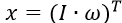, the vector of controls U = u (in the case under consideration it is a scalar), the vector (scalar) of perturbations Mc = f . Matrix model:

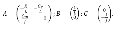(6)

If the rotational speed is chosen as an adjustable value, the measurement equation will be written as:

(7)

and the measurement matrix will take the form:

C = (0 1)

Form the engine model in Python. To do this, we first set specific values ​​for the motor parameters: U = 110 V; R = 0.2 Ohm; L = 0.006 H; J = 0.1 kg / m2; Ce = Cm = 1.3 V / C and we find the values ​​of the coefficient of the object matrices from (6).

Development of a program that generates a model engine with checking matrices for observability and controllability:

When developing the program, the special function def matrix_rank was used to determine the rank of the matrix and the functions listed in the table:

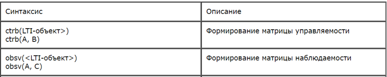
# -*- coding: utf8 -*- from numpy import* from control.matlab import * from numpy.linalg import svd from numpy import sum,where import matplotlib.pyplot as plt def matrix_rank(a, tol=1e-8): s = svd(a, compute_uv=0) return sum( where( s>tol, 1, 0) ) u=110 #   J=.1 #   c=1.3; #   R=.2; L=.006 #      A=matrix([[-R/L ,-c/L],[ c/J ,0]]) print ('  : \n %s'%A) B=matrix([[1/L],[0]]) print (' B : \n %s '%B) C=matrix([[0, 1]]) print (' C : \n %s '%C) D=0 print (' D : \n %s '%D) sd=ss(A,B,C,D) #      wd=tf(sd) #     print ('   : \n %s '%wd) a=ctrb(A,B) print('    : %s'%matrix_rank(a, tol=1e-8)) a=obsv(A,C) print('  : %s'%matrix_rank(a, tol=1e-8)) y,x=step(wd) #    plt.plot(x,y,"b") plt.title('   ') plt.ylabel('    /') plt.xlabel(' ') plt.grid(True) plt.show() 

The results of the program:

Matrix A:
[[-33.33333333 -216.66666667]
[13. 0.]]
Matrix B:
[[166.66666667]
[0.]]
Matrix C:
[[0 1]]
Scalar D:
0
Engine transfer function:
2167 / (s ^ 2 + 33.33 s + 2817)
Rank matrix manageability: 2
Rank Observability Matrix: 2



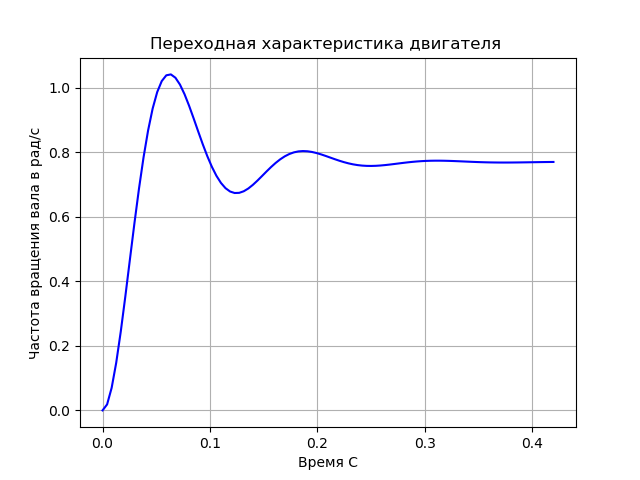
Findings:

1. Using the example of a dc motor with independent magnetic excitation, a technique for designing control in the state space is considered;

2. As a result of the program, the transfer function, transient response, as well as the ranks of the controllability and observability matrices are obtained. The ranks coincide with the dimensions of the state space, which confirms the controllability and observability of the model.

An example of designing an optimal control system with a discrete dlqr controller and full feedback

Definitions and terminology

Linear quadratic regulator (Linear quadratic regulator, LQR) - in the management theory one of the types of optimal regulators using quadratic quality functionality.

The problem in which the system is described by linear differential equations, and the quality indicator is a quadratic functional, is called a linear-quadratic control problem.

Linear quadratic regulators (LQR) and linear quadratic Gaussian regulators (LQG) are widely used.

Getting to the practical solution of the problem, you should always remember the limitations


To synthesize an optimal discrete controller of linear stationary systems, we need a function to solve the Bellman equation. There is no such function in the Python Control Systems library [1], but you can use the function to solve the Riccati equation given in publication [2]:

 def dlqr(A,B,Q,R): """Solve the discrete time lqr controller. x[k+1] = A x[k] + B u[k] cost = sum x[k].T*Q*x[k] + u[k].T*R*u[k] """ #ref Bertsekas, p.151 #first, try to solve the ricatti equation X = np.matrix(scipy.linalg.solve_discrete_are(A, B, Q, R)) #compute the LQR gain K = np.matrix(scipy.linalg.inv(BT*X*B+R)*(BT*X*A)) eigVals, eigVecs = scipy.linalg.eig(AB*K) return K, X, eigVals 

But we must also take into account the restrictions on the synthesis of the optimal regulator, given in [3]:

• the system defined by matrices (A, B) must be stabilized;
• the inequalities S> 0, Q - N / R – NT> 0, the pair of matrices (Q - N / R – NT,
  A - B / R – BT) should not have observable modes with eigenvalues ​​at
  real axis.

After digging into an extensive and not unambiguous theory, which, for obvious reasons, I do not cite, the problem was solved, and all the answers can be read directly in the comments to the code.

The block diagram of the regulator of the control system with feedback on all state variables is shown in the figure:



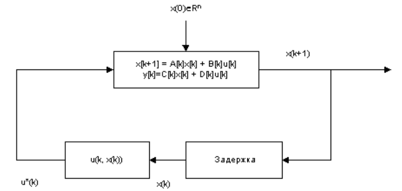
For each initial state x0, the optimal linear controller generates the optimal program control u * (x, k) and the optimal trajectory x * (k).

Program forming optimal control model with dlqr controller

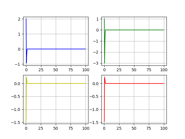
 from numpy import * import scipy.linalg import matplotlib.pyplot as plt def dlqr(A,B,Q,R): #     x[k+1] = A x[k] + B u[k] P= matrix(scipy.linalg.solve_discrete_are(A, B, Q, R)) #  DLQR K = matrix(scipy.linalg.inv(BT*P*B+R)*(BT*P*A)) E, E1 = scipy.linalg.eig(AB*K) return K, P, E """ """ A=matrix([[1, 0],[ -2 ,1]]) B=matrix([[1, 0],[1, 0]]).T """  """ Q=matrix([[0.5, 0],[0, 0.5]]) R=matrix([[0.5,0],[0, 0.5]]) T =100#   SS=0.5#   N =int(T/SS)#   K, P, E=dlqr(A,B,Q,R)#   print("K= \n%s"%K) print("P= \n%s"%P) print("E= \n%s"%E) x = zeros([2, N]) u= zeros([2, N-1]) x [0,0]=2 x [1,0]=1 for i in arange(0,N-2): u[:, i]= dot(- K,x[:, i]) x[:, i+1]=dot(A,x[:, i])+dot(B,u[:, i]) x1= x[0,:] x2= x[1,:] t = arange(0,T,SS) t1=arange(0.5,T,SS) plt.subplot(221) plt.plot(t, x1, 'b') plt.grid(True) plt.subplot(222) plt.plot(t, x2, 'g') plt.grid(True) plt.subplot(223) plt.plot(t1, u[0,:], 'y') plt.grid(True) plt.subplot(224) plt.plot(t1, u[1,:], 'r') plt.grid(True) plt.show() 

Calculation results:

K =
[[0.82287566 -0.17712434]
[0.82287566 -0.17712434]]
P =
[[3.73431348 -1.41143783]
[-1.41143783 1.16143783]]
E =
[0.17712434 + 0.17712434j 0.17712434-0.17712434j]

Dynamics of states and controls: x1, x2, u1, u2.

Conclusion

Separate optimal control problems according to the above can be solved using Python tools, combining the capabilities of the Python Control Systems libraries, SciPy, NumPy, which certainly contributes to the popularization of Python, given that previously such problems could be solved only in paid mathematical packages.

Links

1. Python Control Systems Library.
2. Mark Wilfried Mueller LQR Controllers with Python.
3. E.V. Nikulchev. Manual "Control System Toolbox"