In the previous article about 2048, we used Markov chains to find out that, on average, you need at least 938.8 moves to win, and also investigated the number of possible game field configurations using combinatorics and a full brute force .

In this post, we use a mathematical apparatus called the “Markov Decision Making Process” to find provably optimal strategies for playing 2048 for 2x2 and 3x3 fields, as well as on a 4x4 board up to tile 64 . For example, here’s the optimal player in a 2x2 game before tile 32 :


The random seed determines the random sequence of tiles added by the game on the field. The “strategy” of a player is defined by a table called an algorithm (policy). It tells us in which direction to move the tiles in any possible configuration of the field. In this post we will look at how to create an algorithm that is optimal in the sense that it maximizes the player’s chances of getting a tile 32 .
')
It turns out that in a 2x2 game to tile 32 very difficult to win - even if playing optimally, the player wins only about 8% of cases, that is, the game is not particularly interesting. Qualitatively, 2x2 games are very different from 4x4 games, but they are still useful for getting to know the basic principles.

Ideally, we want to find the optimal algorithm for a full game on a 4x4 field before a 2048 tile, but as we saw from the previous post, the number of possible field configurations is very large. Therefore, it is impossible to create an optimal algorithm for a complete game, at least using the methods used here.

However, we can find the optimal algorithm for the shortened 4x4 game to 64 tile, and, fortunately, we will see that the optimal 3x3 margin game looks qualitatively similar to some successful full-game strategies.

The code (research quality) on which this article is based is laid out in open access .

Markov decision processes for 2048

Markov decision-making processes ( MDP ) are the mathematical basis for modeling and solving problems, in which we need to take a sequence of interconnected solutions under conditions of uncertainty. Such tasks are full in the real world, and the MDP is actively used in economics , financial business and artificial intelligence . In the case of 2048, the sequence of decisions is the direction of movement of the tiles in each move, and uncertainty arises because the game adds tiles to the field at random.

To present the game 2048 in the form of MDP, we need to write it in a certain way. It consists of six basic concepts: states , actions, and transition probabilities encode the dynamics of the game; Rewards , values and algorithms are used to fix the player’s goals and how to achieve them. To develop these six concepts, we take as an example the smallest non-trivial game, similar to 2048, which is played on a 2x2 field only up to tile 8 . Let's start with the first three concepts.

States, actions and transition probabilities

The state fixes the configuration of the field at a given moment of the game, indicating the value of the tile in each of the cells of the field. For example, - This is a possible state in the 2x2 field play. Action is moving left, right, up or down. Every time a player performs an action, the process moves to a new state.

Transition probabilities encode the dynamics of the game, determining the states that are more likely to be next, taking into account the current state and the player’s actions. Fortunately, we can find out exactly how 2048 works by reading its source code . The most important ^one is the process that the game uses to place a random tile on the board. This process is always the same: choose a free cell with the same probability and add a new tile either with a value of 2 with a probability of 0.9, or with a value of 4 with a probability of 0.1 .

At the beginning of each game, using this process, two tiles are added to the field. For example, one of such possible initial states is: . For each action possible in this state, namely L eft, R ight, U p and D own, the possible next states and the corresponding transition probabilities are as follows:


In this diagram, the arrows denote every possible transition to the next state on the right. The weight of the arrow and the label indicate the corresponding transition probability. For example, if a player shifts tiles to the right ( R ), then both tiles 2 move to the right edge, leaving two free cells to the left. A new tile will have a probability of 0.1 tile 4 , and may appear either in the upper left or in the lower left cell, that is, the probability of the state equals $$$0.1 \ times 0.5 = 0.05$ .

From each of these subsequent states, we can continue this process recursively through the search for possible actions and each of their subsequent states. For possible subsequent states are:


Here, a shift to the right is impossible, since none of the tiles can move to the right. Moreover, if a player reaches a subsequent state , highlighted in red, it will lose, because from this state it is impossible to perform valid actions. This will happen if the player performs a left shift, and the game places tile 4 , which happens with a probability of 0.1; from this it can be assumed that a shift to the left is not the best action in this state.

Another last example: if a player moves up, not left, then one of the possible subsequent states will be , and if we iterate over all valid actions and subsequent states from this state, then we can see that a shift to the left or right will lead to tile 8 , which means our victory (highlighted in green):


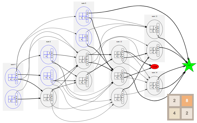
If we repeat this process for all possible initial states and all their possible subsequent states, and so on recursively, until we reach a win or lose state, we can build a complete model with all possible states, actions and their transition probabilities. For a 2x2 game up to tile 8 this model looks like this ( click to enlarge ; you may have to scroll down the page):


To make the scheme smaller, all loss states need to be reduced to a single state lose , shown by a red oval, and all winning states should be similarly reduced to a single win state shown by a green star. This is possible because in fact we are not interested in how the player won or lost, but the result itself is important.

The game proceeds approximately in the diagram from left to right, because the states are ordered into “layers” by the sum of their tiles. The useful feature of the game is that after each action the amount of tiles on the field increases by 2 or 4. This happens because merging tiles does not change the amount of tiles on the field, and the game always adds either 2 or 4 . The possible initial states, which are layers with a sum of 4, 6, and 8, are shown in blue.

Even in the model of such a minimal example, 70 states and 530 transitions. However, these values ​​can be significantly reduced by noting that many of the states we have listed are trivially related to rotations and reflections, as described in Appendix A. In practice, this observation is very important for reducing the size of the model and effectively solving it. In addition, it allows you to create more convenient schemes, but for the transition to the second set of concepts of a Markov decision-making process is not necessary.

Rewards, Values ​​and Algorithms

To complete the specification of the model, we need to somehow encode the fact that the player’s goal is to achieve a win ² state. We will do this by defining the rewards . In general, each time MDP enters a state, the player receives a reward depending on the state. We assign the reward for the transition to the win state to 1, and for the transition to other states - the value of 0. That is, the only way to get a reward is to reach the win state ³ .

Now that we have a MDP model of the game, described with respect to states, actions, transition probabilities and rewards, we are ready to solve it. An MDP solution is called an algorithm . In essence, this is a table in which for each possible state an action is indicated that needs to be performed in this state. Solving an MDP means finding the optimal algorithm , that is, one that allows the player to get as much reward as possible over time.

To make it accurate, we need the last MDP concept: the value of a state according to a given algorithm is the expected reward the player will receive if he starts from this state and then follows the algorithm. Some records are needed to explain this.

Let be $$$S$ Is a set of states, and for each state $$$s \ in S$$$$A_s$ will be a set of actions allowed in the state $$$s$ . Let be $$$\ Pr (s ’| s, a)$ denotes the probability of transition to each subsequent state $$$s ’\ in S$ , given that the process is in a state $$$s \ in S$ and the player performs the action $$$a \ in A_s$ . Let be $$$R (s)$ denotes reward for transition to the state $$$s$ . Finally let $$$\ pi$ mean algorithm as well $$$\ pi (s) \ in A_s$ denotes the action to be performed in the state $$$s$ to follow the algorithm $$$\ pi$ .

For a given algorithm $$$\ pi$ and states $$$s$ state value $$$s$ according to $$$\ pi$ equally

$$

$$V ^ \ pi (s) = R (s) + \ gamma \ sum_ {s ’} \ Pr (s’ | s, \ pi (s)) V ^ \ pi (s ’)$$

where the first term is an instantaneous reward, and summation gives the expected value of the subsequent states, provided that the player continues to follow the algorithm.

Coefficient $$$\ gamma$ - is the depreciation rate , which replaces the value of the instantaneous remuneration by the value of the expected future remuneration. In other words, it takes into account the cost of money, taking into account the time factor : the reward now usually costs more than the same reward later. If a $$$\ gamma$ close to 1, this means that the player is very patient: he does not mind waiting for a future reward; similarly, smaller values $$$\ gamma$ mean the player is less patient. For now, we assign the depreciation factor $$$\ gamma$ a value of 1, which corresponds to our assumption that the player cares only about the victory, and not the time it takes for her ⁴ .

So how do we find an algorithm? In each of the states, we want to choose an action that maximizes the expected future reward:

$$

$$\ pi (s) = \ mathop {\ mathrm {argmax}} \ limits_ {a \ in A_s} \ left \ {\ sum_ {s '} \ Pr (s' | s, a) V ^ \ pi (s ') \ right \}$$

This gives us two related equations that we can solve iteratively. That is, choose the original algorithm, which can be very simple, calculate the value of each state in accordance with this simple algorithm, and then find a new algorithm based on this function of values, and so on. It is noteworthy that in very limited technical conditions such an iterative process is guaranteed to converge to the optimal algorithm. $$$\ pi ^ *$ and optimal function of values $$$V ^ {\ pi ^ *}$ regarding this optimal algorithm.

Such a standard iterative approach works well for models of MDP games on a 2x2 field, but is not suitable for models of 3x3 and 4x4 games that have much more states and therefore consume much more memory and computing power. Fortunately, it turns out that we can use the structure of our 2048 models for a much more efficient solution of these equations (see Appendix B).

The optimal game on the field 2x2

Now we are ready to see the optimal algorithms in action! If you enter the initial number 42 and press the Start button in the original article, you will reach tile 8 in 5 moves. The initial number determines the sequence of new tiles placed by the game; if you select a different starting number by pressing the button, then (usually) the game will evolve differently.


In the game 2x2 before tile 8 really nothing to look at. If the player follows the optimal algorithm, he will always win. (As we saw above when building transition probabilities, if a player plays suboptimally, that is, the possibility of losing.) This is reflected in the fact that the value of the state throughout the game remains equal to 1.00 - with an optimal game there is at least one action in each attainable state, which leads to victory.

If we instead ask the player to play before tile 16 , then even with an optimal game, the victory will no longer be guaranteed. In this case, when playing before tile 16 choice of a new initial number should lead to victory in 96% of cases, so we have chosen one of the few that lead to loss as the initial number.


As a result of the assignment of the depreciation factor $$$\ gamma$ Values ​​1 The value of each state tells us the probability of winning from this state. Here the value starts from 0.96, and then gradually decreases to 0.90, because the outcome depends on whether the next tile will have the value 2 . Unfortunately, the game sets tile 4 , so the player loses, despite the optimal game.

Finally, we have previously established that the largest attainable tile on a 2x2 field is tile 32 , so let's look at the optimal algorithm. Here, the probability of winning drops to only 8%. (This is the same game and the same algorithm used in the introduction, but now interactive.)


It is worth noting that each of the algorithms shown above is the optimal algorithm of the corresponding game, but there is no guarantee of its uniqueness. There may be many similar optimal algorithms, but we can definitely say that none of them is strictly the best.

If you want to explore these models for the 2x2 game in more detail, then Appendix A contains diagrams showing all possible paths to the game.

The optimal game on the field 3x3

On the 3x3 field, you can play up to 1024 tiles, and this game has 25 million states . Therefore, it is absolutely impossible to draw the MDP scheme, which we did for 2x2 games, but we can still observe the optimal algorithm in action ⁵ :


Just like in the 2x2 game to tile 32 , in the 3x3 game to 1024 tile it is very difficult to win - with an optimal game, the probability of winning is only about 1%. As a less useless entertainment, you can choose a game before tile 512 , in which the probability of winning with an optimal game is much higher, about 74%:


At the risk of anthropomorphic large state and action tables, which is the algorithm, I see here elements of the strategies that I use when playing in 2048 on a 4x4 field. We see that the algorithm puts tiles with high values ​​on the edges and usually in corners (although in the game up to 1024 he often places a tile 512 in the middle of the field boundary). You can also notice that he is "lazy" - even when there are two tiles with high values ​​that can be combined, he continues to combine values ​​with smaller values. It is logical that, especially in the cramped 3x3 field conditions, it is worth using the opportunity to increase the amount of your tiles without the risk of (instantaneous) loss - if it fails to combine smaller tiles, it can always combine larger ones, which frees the field.

It is important to note that they did not train the algorithm in these strategies and did not give him any hints.
about how to play. All his behaviors and apparent intelligence arise exclusively from the solution of the optimization problem, taking into account the transition probabilities and the reward function transferred by us.

The best game on the field 4x4

As it turned out in the previous post, the game before the 2048 tile on the 4x4 field has at least trillions of states, so it is not yet possible to even list all the states, let alone the MDP solution, to obtain the optimal algorithm.

However, we can iterate over and execute the solution for a 4x4 game to a tile of 64 — there will be “only” 40 billion states in this model. As in the game 2x2 before tile 8 , with optimal play it is impossible to lose. Therefore, it is not very interesting to observe it, since in many cases there are several good states, and the choice between them is carried out in an arbitrary manner.

However, if we reduce the depreciation rate $$$\ gamma$ that will make the player a little impatient, he will prefer to win faster rather than later. Then the game will look a little more targeted. Here is the optimal player when $$$\ gamma = 0.99$ :


Initially, the value is approximately 0.72; the exact initial value reflects the expected number of steps that will be required to win from a randomly selected initial state. It gradually increases with each turn, because the reward for achieving the state of victory becomes closer. The algorithm again makes good use of the borders and corners of the field to build sequences of tiles in a convenient way to merge.

Conclusion

We figured out how to present the 2048 game as a Markov decision-making process and obtained demonstrably optimal algorithms for the 2x2 and 3x3 field games, as well as for the limited game on the 4x4 field.

The methods used here require a solution to enumerate all the states of the model. The use of effective state transfer strategies and effective strategies for solving this model (see Appendix B) makes them suitable for models with up to 40 billion states, that is, for playing 4x4 to 64 . Calculations for this model required approximately one week of operation of the OVH HG-120 instance with 32 cores, 3.1 GHz and 120GB of RAM. The next closest 4x4 game to tile 128 is likely to contain many times more states and will require much more computing power.Calculating a provably optimal algorithm for a full game up 2048probably will require other methods of solution.

It often turns out that MDP in practice is too large to be solved, therefore there are proven techniques for finding approximate solutions. They usually use the storage of approximate functions of values ​​and / or algorithm, for example, using learning (possibly deep) neural networks. Also, instead of listing the entire state space, they can be trained on these simulations using reinforced learning methods. The existence of demonstrably optimal algorithms for smaller games can make the 2048 a useful test bed for such methods - this can be an interesting topic for research in the future.

---

Appendix A: canonization

As we saw in the example of the full model for a 2x2 game to a tile 8, the number of states and transitions grows very quickly, and it becomes difficult to graphically present even games on a 2x2 field.

To maintain control over the size of the model, we can again use the observation from the previous post about the enumeration of states : many of the subsequent states are simply turns and reflections of each other. For example, states


and

they are just mirror copies — they are just reflections on the vertical axis. If the best action in the first state is a shift to the left, then the best action in the second state will necessarily be a shift to the right. That is, from the point of view of making decisions about the choice of an action, it suffices to choose one of the states as canonical and determine the best action that needs to be made from the canonical state. The canonical state of a given state is obtained by finding all its possible turns and reflections, recording each one as the number on the base 12 and selecting the state on the smallest number — see details in the previous post.. It is important here that each canonical state replaces the class of equivalent states associated with it by rotation or reflection, so we will not have to deal with them separately. Replacing the subsequent states presented above with their canonical states, we obtain a more compact scheme:


Unfortunately, from the scheme it follows that a shift up ( U) from some way will lead to . However, the paradox is resolved by reading the arrows and adding a rotation or reflection if necessary, in order to find the actual canonical state of the subsequent state.

Equivalent actions

We can also note that in the diagram shown above, in fact, it does not matter in which direction the player performs a shift from the state — the canonical successive states and their transition probabilities are the same for all actions. To understand why, it is worth looking at the “intermediate state” after the player has made a shift to move the tiles, but when the game has not yet added a new random tile:


Intermediate states are marked with dashed lines. The most important thing to notice here is that they are all connected by a 90 ° rotation. These twists and turns are not important if, as a result, we canonize subsequent states.

More generally, if two or more actions have the same canonical “intermediate state”, then these actions must have the same canonical successive states, and therefore they are equivalent. In the example shown above, the last canonical intermediate state is: .

Therefore, we can further simplify the scheme for if we simply combine all the equivalent actions:



Of course, states for which all actions are equivalent in this sense are relatively rare. Having considered another potential initial state , we will see that the left and right shifts are equivalent, but the upward shift is different; a down shift is not allowed because the tiles are already at the bottom.

MDP Models for 2x2 Games

Thanks to canonization, we can reduce the model to a scale at which you can draw full MDP for some small games. Let's start again with the smallest non-trivial model: 2x2 games to the tile 8:


Compared to the scheme without canonization, this one turned out to be much more compact. We see that the shortest possible game consists of only one move: if we are lucky to start from a state with two adjacent tiles 4, which happens only in one game for 150, we just need to connect them to get a tile 8and a state win. On the other hand, we see that it is still possible to lose: if from the state the player shifts upwards, then with a probability of 0.9 he will receiveif it makes a shift again, it will receive with a probability of 0.9 , and at that moment the game will be lost.

We can further simplify the scheme if we know the optimal algorithm. The definition of the algorithm generates a Markov chain from the MDP model, because each state has a single action or a group of equivalent actions defined by the algorithm. The generated chain for a 2x2 game 8has the following form:


We see that loseno more edges lead to the state , because with an optimal game of 2x2 before the tile, 8it is impossible to lose. In addition, each state is now marked with its value, which in this case is always equal to 1.000. Since we assigned the depreciation rate$$γ value is 1, then the value of the state is actually the probability of gaining from this state in the optimal game. The schemes become a bit more chaotic, but we can build similar models for playing 2x2 tiles:$\gamma$

16


If we look at the optimal algorithm for the game to the tile 16, we see that the initial states (blue) have values ​​less than one, and that there are paths to the state lose, in particular, from two states in which the sum of tiles is 14:


That is, if we play this game before the tile in the 16optimal way, we will still be able to lose, and this will depend on the specific sequence of the tiles given to us by the game 2and 4. However, in most cases we will win - the values ​​in the initial states are approximately equal to 0.96, so we expect to win in about 96 games out of a hundred.

However, our prospects for playing up 32to a 2x2 tile on the field are much worse. Here is the complete model:


We see that many edges lead to a state lose, and this is a bad sign. This is confirmed, if you look at the scheme, limited to the optimal game:


The average value for the initial states is approximately 0.08, so we should expect victory in about 8 games out of a hundred. The main reason for this becomes apparent when we look at the right side of the diagram: reaching a state with a sum of 28, the only way to win is to get a tile 4to reach the state .If we get a tile 2, which happens 90% of the time, we lose. Perhaps this game will not be very interesting.

Appendix B: Solution Methods

To effectively solve MDP models that are similar to the ones we built here for 2048, we can use the important properties of their structure:

1. (). , — 2 4, .
2. , «» , MDP, $$$s$ $$$s+2$ , , $$$s+4$ .
3. , , 0 1.

Property (3) means that we can loop through all the states in the last layer, in which all subsequent values ​​are known, and generate a function of values ​​for this last layer. Further, thanks to property (2), we know that the states in the second from the end of the layer must go either to the states in the last layer for which we have just calculated the values, or to the win or lose state, which have known values. In this way, we can go backwards, layer by layer, always knowing the values ​​of the states in the next two layers; this allows us to construct both a function of values ​​and an optimal algorithm for the current layer.

In the previous postwe did the work in a straightforward order, from the initial states and enumerated all the states, layer by layer, using a convolution mapping to parallelize the work inside each layer. For the solution, we can use the output of this enumeration, which is a huge list of states, to perform the work in the reverse order, again applying a convolution mapping for parallel work in each layer. Like last time, we split the layers into “parts” according to their maximum tile values ​​with tracking additional information.

Basic solver implementationit is still quite memory demanding, because in order to process the current part in one pass, it needs to store in memory the functions of several (up to four) parts. You can reduce this requirement until only one part is stored in memory at one time by what is commonly called$$Q π ( s , a ) - values ​​for each possible state-action pair according to the algorithm$Q^\pi(s,a)$$$π and not$\pi$$$V π ( s ) , butthis implementation of the solverturned out to be much slower, so all the results were obtained using the main solver$V^\pi(s)$$$V π on a machine with a lot of RAM.In the case of both solvers, the layered structure of the model allows us to build and solve a model with just one pass forward and one pass back, which is a significant improvement over the conventional iterative solution method. This is one of the reasons why we are able to solve such fairly large MDP models with billions of states. Also important reasons are the methods of canonization from Appendix A, which allow to reduce the number of counted states, andlow-level efficiency optimizationfrom the previous post.$V^\pi$

---

I thank Hope Thomas for editing the drafts of this article.

If you've read this far, then you might want to subscribe to my twitter , or even send your resume to work at Overleaf .

Notes

1. : , 2 , , , 4 , 8 . . , , , ( ) — ; .
2. dot graphviz .
3. . , 2048 ; , . , . , 1 , , , .
4. , , win lose . , $$$\pi$ and $$$V^\pi$ , , , lose win . end , end 1. lose win , end 1. end , . , MDP, , , , , ( : , .
5. , , . , . , , . , , 1, , , .
6. 3x3 4x4 : ( , GitHub, ). , $$$10^{-7}$ . , , , , , , . , . , 2048 .
7. , , 2048. !