About streams and tables in Kafka and Stream Processing, part 1
* Michael G. Noll is an active contributor to Open Source projects, including Apache Kafka and Apache Storm.
The article will be useful primarily for those who are just acquainted with Apache Kafka and / or stream processing.
In this article, perhaps in the first of a mini-series, I want to explain the concepts of Streams and Tables in stream processing and, in particular, in Apache Kafka . I hope you will have a better theoretical presentation and ideas that will help you solve your current and future tasks better and / or faster.
')
Content:
* Motivation
* Streams and Tables in simple language
* Illustrated examples
* Streams and Tables in Kafka in simple language
* A closer look at Kafka Streams, KSQL and analogues in Scala
* Tables stand on the shoulders of giants (on streams)
* Turning the Database Inside-Out
* Conclusion
In my daily work, I communicate with many Apache Kafka users and those who do streaming with Kafka through Kafka Streams and KSQL (streaming SQL for Kafka). Some users already have experience in stream processing or using Kafka, some have experience using RDBMS, such as Oracle or MySQL, some have neither one nor the other experience.
A frequently asked question: “What is the difference between streams and tables?” In this article I want to give both answers: both short (TL; DR) and long, so that you can get a deeper understanding. Some of the explanations below will be slightly simplified, because it simplifies understanding and memorization (for example, as a simpler model of Newton's attraction is quite sufficient for most everyday situations, which saves us from having to go directly to Einstein’s relativistic model, but so complicated).
Another common question: “Well, but why should I care? How will this help me in my daily work? ”In short, for many reasons! As you begin to use stream processing, you will soon realize that in practice, in most cases, both streams and tables are required. Tables, as I will explain later, represent a state. Whenever you perform any processing with [stateful processing] , such as joins (for example, enriching data [ data enrichment ] in real time by combining the flow of facts with dimension tables [ dimension tables ] ) or aggregation ] (for example, real-time calculation of the average for key business indicators in 5 minutes), then the tables introduce a streaming picture. Otherwise, this means that you will have to do it yourself [a lot of DIY pain] .
Even the notorious WordCount example, probably your first “Hello World” from this area, falls into the “with state” category: this is an example of processing with a state where we aggregate a stream of rows into a continuously updated table / map to count words. Thus, regardless of whether you implement WordCount streaming or something more complicated, like fraud detection , you want an easy-to-use streaming solution with basic data structures and everything you need inside (hint: streams and tables ). You certainly don’t want to build a complex and unnecessary architecture where you need to combine (only) stream processing technology with remote storage, such as Cassandra or MySQL, and possibly with the addition of Hadoop / HDFS to ensure fault tolerance processing [fault-tolerance processing ] (three things - too much).
Here is the best analogy I could come up with:
And as an aperitif to the future post: if you have access to the entire history of events in the world (stream), then you can restore the state of the world at any time , that is, a table at an arbitrary time
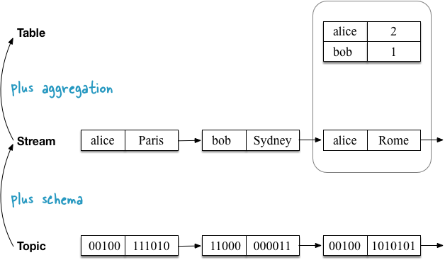
The first example shows a stream with geo-locations of users that are aggregated into a table fixing the current (last) position of each user . As I will explain later, this also turns out to be the default semantics for tables when you read the [Topic] Kafka topic directly into the table.
The second usage example demonstrates the same stream of user geolocation updates, but now the stream is aggregated into a table that records the number of places visited by each user . Since the aggregation function is different (here: counting the number), the table contents are also different. More precisely, other values by key.

Before we get into the details, let's start with a simple one.
A topic in Kafka is an unlimited sequence of key-value pairs. Keys and values are ordinary byte arrays, i.e.
Stream is a topic with a schema . Keys and values are no longer arrays of bytes, but have a specific type.
A table is a table in the usual sense of the word (I feel the joy of those of you who are already familiar with RDBMS and are just getting acquainted with Kafka). But looking through the prism of stream processing, we see that the table is also an aggregated stream (you really didn’t expect us to dwell on the definition “table is a table”, is it?).
Total:
Topics, streams and tables have the following properties in Kafka:
Let's look at how topics, streams, and tables relate to the Kafka Streams API and KSQL, as well as draw analogies with programming languages (it is ignored in analogies, for example, that topics / streams / tables can be partitioned):
But this summary at this level may be of little use to you. So let's take a closer look.
I will start each of the following sections with the analogy in Scala (imagine that stream processing is done on the same machine) and the Scala REPL so that you can copy the code and play with it yourself, then I will explain how to do the same in Kafka Streams and KSQL (flexible, scalable and fault tolerant stream processing on distributed machines). As I mentioned at the beginning, I simplify the explanations below a little. For example, I will not consider the influence of partitioning in Kafka.
A topic in Kafka consists of key-value messages. The topic does not depend on the serialization format or the “type” of messages: the keys and values in the messages are treated as ordinary
Kafka Streams and KSQL do not have a “topic” concept. They only know about streams and tables. Therefore, I will show here only an analogue of the topic in Scala.
Now we are reading the topic in the stream, adding information about the schema (schema for reading [schema-on-read] ). In other words, we turn a raw, untyped topic into a “typed topic” or stream.
In Scala, this is achieved using the
In Kafka Streams, you read the topic in
In KSQL, you have to do something like the following in order to read the topic as
Now we are reading the same topic in the table. First, we need to add schema information (a schema for reading). Secondly, you must convert the stream to a table. The semantics of the table in Kafka states that the final table should map each message key from the topic to the last value for that key.
Let's first use the first example, where the summary table tracks the last location of each user:
In Scala:
Adding information about the scheme is achieved using the first
What is interesting about the relationship between streams and tables is that the command above creates a table equivalent to the short version below (remember referential transparency ), where we build the table directly from the stream, which allows us to skip the schema / type setting because the stream is already typed. We can see that the table is derivation , stream aggregation :
In Kafka Streams, you usually use
But for clarity, you can also read the topic first in
In KSQL, you have to do something like the following in order to read the topic as
What does this mean? This means that the table is actually an aggregated stream , as we said at the very beginning. We saw this directly in the special case above, when the table was created directly from the topic. However, this is actually the general case.
Conceptually, only stream is the construction of first-order data in Kafka. On the other hand, the table is either (1) derived from an existing stream by means of a key [per-key] aggregation, or (2) is derived from an existing table, which always expands to an aggregated stream (we could call the last tables “protostream” [ "Ur-stream"] ).
Of the two cases, the more interesting discussion is (1), so let's focus on that. And this probably means that I need to first figure out how the aggregation works in Kafka.
Aggregation is one type of stream processing. Other types, for example, include filtering [filters] and joins [joins] .
As we found out earlier, the data in Kafka are presented in the form of key-value pairs. Further, the first property of aggregations in Kafka is that they are all calculated by key . That is why we have to group
The second property of aggregations in Kafka is that aggregations are continuously updated as soon as new data enters the incoming streams. Together with the property of computing by key, this requires the presence of a table or, more precisely, it requires a mutable table as a result and, therefore, the type of returned aggregations. Previous values (aggregation results) for the key are constantly overwritten with new values. Both in Kafka Streams and in KSQL, aggregations always return a table.
Let us return to our second example, in which we want to calculate, by our flow, the number of places visited by each user:
Counting is the type of aggregation. To calculate the values, we only need to replace the aggregation stage from the previous section
The code on Kafka Streams is equivalent to the Scala example above:
In KSQL:
As we saw above, tables are aggregations of their input streams, or, in short, tables are aggregated streams. Whenever you perform an aggregation in Kafka Streams or KSQL, the result is always a table.
The feature of the aggregation stage determines whether the table is directly retrieved from the stream via UPSERT stateless semantics (the table maps the keys to their last value in the stream, which is aggregation when reading the Kafka topic directly into the table), by counting the number of seen values for each key [stateful counting] states (see our last example), or more complex aggregations, such as summation, averaging, and so on. When using Kafka Streams and KSQL, you have many options for aggregation, including windowed aggregations with “tumbling windows”, “hopping” windows, and “session” windows.
Although the tables is an input stream aggregation, it also has its own output stream! Like change data records (CDC) in databases, every change in a table in Kafka is recorded in an internal stream of changes called the changelog stream table. Many calculations in Kafka Streams and KSQL are actually performed on the changelog stream . This allows Kafka Streams and KSQL, for example, to correctly process historical data in accordance with the semantics of event time processing [event-time processing semantics] - remember that the stream represents both the present and the past, while the table can represent only the present (or, more precisely, the fixed moment of time [snapshot in time] ).
Here is the first example, but now with the changelog stream :
Please note that the changelog stream of the table is a copy of the input stream of this table. This is due to the nature of the corresponding aggregation function (UPSERT). And if you're wondering: “Wait, isn't it 1 to 1 copying, wasting disk space?” - Under the hood, Kafka Streams and KSQL are optimized to minimize unnecessary data copying and local / network IO. I ignore these optimizations in the diagram above to better illustrate what is happening in principle.
And finally, a second usage example, which includes the changelog stream . Here the stream of table changes is different, because here is another aggregation function that performs per-key counts.

But these internal changelog streams also have an architectural and operational impact. The streams of changes are continuously backed up and saved as topics in Kafka, and the topic itself is part of the magic that provides elasticity and resiliency in Kafka Streams and KSQL. This is due to the fact that they allow you to move processing tasks between machines / virtual machines / containers without losing data and for all operations, regardless of whether the processing is with [stateful] or without [stateless] . The table is part of the state [state] of your application (Kafka Streams) or query (KSQL), so Kafka is required to transfer not only processing code (which is easy), but also processing states, including tables, between machines in a fast and reliable way ( which is much more complicated). Whenever the table has to be moved from client machine A to machine B, then on a new assignment B the table is reconstructed from its changelog stream to Kafka (on the server side) the exact same state as on machine A. We can see it on The last diagram above, where the “ counting table” [] can be easily restored from its changelog stream without the need to recycle the input stream.
The term stream-table duality refers to the above relationship between streams and tables. This means, for example, that you can turn a stream into a table, this table into another stream, a received stream into another table, and so on. For more information, see the Confluent blog post: Introduction to Kafka Streams: Stream Processing Made Simple .
In addition to what we covered in the previous sections, you may have come across the Turning the Database Inside-Out article, and now you might be interested in looking at this in its entirety? Since I don’t want to go into details now, let me briefly compare the world of Kafka and stream processing with the world of databases. Be vigilant: further, black-and-white simplifications .
In databases, the table is a first-order construction. This is what you work with. “Streams” also exist in databases, for example, in the form of a binlog in MySQL or GoldenGate in Oracle , but they are usually hidden from you in the sense that you cannot interact with them directly. The database is aware of the present, but it does not know about the past (if you need the past, recover data from your backup tapes , which, ha ha, just hardware streams).
In Kafka and stream processing, stream is a first order construct. Tables are derivatives of streams [derivations of streams] , as we have seen before. Stream knows about the present and about the past. As an example, the New York Times keeps all published articles - 160 years of journalism from the 1850s - at Kafka, the source of reliable data.
In short: the database thinks first with a table, and then with a stream. Kafka thinks first with stream and then with the table. , Kafka- , , — , WordCount, , . , Kafka , Kafka Streams KSQL, ( ). Kafka , , - [stream-relational] , [stream-only].
, , Kafka . , , « » « Kafka ».
- Kafka, Kafka Streams KSQL, :
, Kafka Streams KSQL, Kafka , , (, , , , , , ). , . :-)
, « , 1». , , . ? !
— , , .
The article will be useful primarily for those who are just acquainted with Apache Kafka and / or stream processing.
In this article, perhaps in the first of a mini-series, I want to explain the concepts of Streams and Tables in stream processing and, in particular, in Apache Kafka . I hope you will have a better theoretical presentation and ideas that will help you solve your current and future tasks better and / or faster.
')
Content:
* Motivation
* Streams and Tables in simple language
* Illustrated examples
* Streams and Tables in Kafka in simple language
* A closer look at Kafka Streams, KSQL and analogues in Scala
* Tables stand on the shoulders of giants (on streams)
* Turning the Database Inside-Out
* Conclusion
Motivation, or why should it care?
In my daily work, I communicate with many Apache Kafka users and those who do streaming with Kafka through Kafka Streams and KSQL (streaming SQL for Kafka). Some users already have experience in stream processing or using Kafka, some have experience using RDBMS, such as Oracle or MySQL, some have neither one nor the other experience.
A frequently asked question: “What is the difference between streams and tables?” In this article I want to give both answers: both short (TL; DR) and long, so that you can get a deeper understanding. Some of the explanations below will be slightly simplified, because it simplifies understanding and memorization (for example, as a simpler model of Newton's attraction is quite sufficient for most everyday situations, which saves us from having to go directly to Einstein’s relativistic model, but so complicated).
Another common question: “Well, but why should I care? How will this help me in my daily work? ”In short, for many reasons! As you begin to use stream processing, you will soon realize that in practice, in most cases, both streams and tables are required. Tables, as I will explain later, represent a state. Whenever you perform any processing with [stateful processing] , such as joins (for example, enriching data [ data enrichment ] in real time by combining the flow of facts with dimension tables [ dimension tables ] ) or aggregation ] (for example, real-time calculation of the average for key business indicators in 5 minutes), then the tables introduce a streaming picture. Otherwise, this means that you will have to do it yourself [a lot of DIY pain] .
Even the notorious WordCount example, probably your first “Hello World” from this area, falls into the “with state” category: this is an example of processing with a state where we aggregate a stream of rows into a continuously updated table / map to count words. Thus, regardless of whether you implement WordCount streaming or something more complicated, like fraud detection , you want an easy-to-use streaming solution with basic data structures and everything you need inside (hint: streams and tables ). You certainly don’t want to build a complex and unnecessary architecture where you need to combine (only) stream processing technology with remote storage, such as Cassandra or MySQL, and possibly with the addition of Hadoop / HDFS to ensure fault tolerance processing [fault-tolerance processing ] (three things - too much).
Stream and Tables in simple language
Here is the best analogy I could come up with:
- Stream in Kafka is the complete history of all the events that have happened (or just business events) in the world from the beginning of time to the present day . He represents the past and present. As we move from today to tomorrow, new developments are constantly added to world history.
- The table in Kafka is a state of the world today . She is present. It is the aggregation of all the events in the world that is constantly changing as we move from today to tomorrow.
And as an aperitif to the future post: if you have access to the entire history of events in the world (stream), then you can restore the state of the world at any time , that is, a table at an arbitrary time
t in the stream, where t not limited to only t= In other words, we can create “snapshots” of the state of the world (table) at any time point t , for example, 2560 BC, when the Great Pyramid was built at Giza, or 1993, when the European UnionIllustrated examples
The first example shows a stream with geo-locations of users that are aggregated into a table fixing the current (last) position of each user . As I will explain later, this also turns out to be the default semantics for tables when you read the [Topic] Kafka topic directly into the table.
The second usage example demonstrates the same stream of user geolocation updates, but now the stream is aggregated into a table that records the number of places visited by each user . Since the aggregation function is different (here: counting the number), the table contents are also different. More precisely, other values by key.
Stream and Tables in Kafka in simple language
Before we get into the details, let's start with a simple one.
A topic in Kafka is an unlimited sequence of key-value pairs. Keys and values are ordinary byte arrays, i.e.
<byte[], byte[]> .Stream is a topic with a schema . Keys and values are no longer arrays of bytes, but have a specific type.
Example:<byte[], byte[]>topic is read as<User, GeoLocation>stream user geolocation.
A table is a table in the usual sense of the word (I feel the joy of those of you who are already familiar with RDBMS and are just getting acquainted with Kafka). But looking through the prism of stream processing, we see that the table is also an aggregated stream (you really didn’t expect us to dwell on the definition “table is a table”, is it?).
Example:<User, GeoLocation>stream with geodata updates is aggregated into a<User, GeoLocation>table, which tracks the user's last position. At the aggregation stage, [UPSERT] values in the table are updated according to the key from the input stream. We saw this in the first illustrated example above.
Example:<User, GeoLocation>stream is aggregated into<User, Long>table, which tracks the number of visited locations for each user. At the stage of aggregation, values are continuously calculated (and updated) by keys in the table. We saw this in the second illustrated example above.
Total:
Topics, streams and tables have the following properties in Kafka:
| Type of | There are partitions | Is not limited | There is order | Changeable | Key uniqueness | Scheme |
|---|---|---|---|---|---|---|
| Topic | Yes | Yes | Yes | Not | Not | Not |
| Stream | Yes | Yes | Yes | Not | Not | Yes |
| Table | Yes | Yes | Not | Yes | Yes | Yes |
Let's look at how topics, streams, and tables relate to the Kafka Streams API and KSQL, as well as draw analogies with programming languages (it is ignored in analogies, for example, that topics / streams / tables can be partitioned):
| Type of | Kafka streams | KSQL | Java | Scala | Python |
|---|---|---|---|---|---|
| Topic | - | - | List / Stream | List / Stream [(Array[Byte], Array[Byte])] | [] |
| Stream | KStream | STREAM | List / Stream | List / Stream [(K, V)] | [] |
| Table | KTable | TABLE | HashMap | mutable.Map[K, V] | {} |
But this summary at this level may be of little use to you. So let's take a closer look.
A closer look at Kafka Streams, KSQL and analogues in Scala
I will start each of the following sections with the analogy in Scala (imagine that stream processing is done on the same machine) and the Scala REPL so that you can copy the code and play with it yourself, then I will explain how to do the same in Kafka Streams and KSQL (flexible, scalable and fault tolerant stream processing on distributed machines). As I mentioned at the beginning, I simplify the explanations below a little. For example, I will not consider the influence of partitioning in Kafka.
If you do not know Scala: Do not be embarrassed! You do not need to understand Scala analogs in all details. It is enough to pay attention to what operations (for example,map()) are connected together, what they are (for example,reduceLeft()is an aggregation), and how the “chain” of streams relates to the “chain” of tables.
Topics
A topic in Kafka consists of key-value messages. The topic does not depend on the serialization format or the “type” of messages: the keys and values in the messages are treated as ordinary
byte[] arrays. In other words, from this point of view, we have no idea what is inside the data.Kafka Streams and KSQL do not have a “topic” concept. They only know about streams and tables. Therefore, I will show here only an analogue of the topic in Scala.
// Scala analogy scala> val topic: Seq[(Array[Byte], Array[Byte])] = Seq((Array(97, 108, 105, 99, 101),Array(80, 97, 114, 105, 115)), (Array(98, 111, 98),Array(83, 121, 100, 110, 101, 121)), (Array(97, 108, 105, 99, 101),Array(82, 111, 109, 101)), (Array(98, 111, 98),Array(76, 105, 109, 97)), (Array(97, 108, 105, 99, 101),Array(66, 101, 114, 108, 105, 110))) Streams
Now we are reading the topic in the stream, adding information about the schema (schema for reading [schema-on-read] ). In other words, we turn a raw, untyped topic into a “typed topic” or stream.
Schema for reading vs Schema for writing [schema-on-write] : Kafka and its topics do not depend on the serialization format of your data. Therefore, you must specify a schema when you want to read the data in a stream or table. This is called a read scheme . The reading scheme has both advantages and disadvantages. Fortunately, you can choose an intermediate between a read scheme and a write scheme, defining a contract for your data — much like you probably define API contracts in your applications and services. This can be achieved by choosing a structured, but extensible data format, such as Apache Avro, with a roll -out of the registry for your Avro-schemas, such as Confluent Schema Registry . And yes, both Kafka Streams and KSQL support Avro, if you're interested.
In Scala, this is achieved using the
map() operation below. In this example, we get a stream from the <String, String> pairs. Notice how we can now look inside the data. // Scala analogy scala> val stream = topic | .map { case (k: Array[Byte], v: Array[Byte]) => new String(k) -> new String(v) } // => stream: Seq[(String, String)] = // List((alice,Paris), (bob,Sydney), (alice,Rome), (bob,Lima), (alice,Berlin)) In Kafka Streams, you read the topic in
KStream via StreamsBuilder#stream() . Here you have to define the desired scheme using the Consumed.with() parameter when reading data from the topic: StreamsBuilder builder = new StreamsBuilder(); KStream<String, String> stream = builder.stream("input-topic", Consumed.with(Serdes.String(), Serdes.String())); In KSQL, you have to do something like the following in order to read the topic as
STREAM . Here you define the desired scheme by specifying the names and types of columns when reading data from the topic: CREATE STREAM myStream (username VARCHAR, location VARCHAR) WITH (KAFKA_TOPIC='input-topic', VALUE_FORMAT='...') Tables
Now we are reading the same topic in the table. First, we need to add schema information (a schema for reading). Secondly, you must convert the stream to a table. The semantics of the table in Kafka states that the final table should map each message key from the topic to the last value for that key.
Let's first use the first example, where the summary table tracks the last location of each user:
In Scala:
// Scala analogy scala> val table = topic | .map { case (k: Array[Byte], v: Array[Byte]) => new String(k) -> new String(v) } | .groupBy(_._1) | .map { case (k, v) => (k, v.reduceLeft( (aggV, newV) => newV)._2) } // => table: scala.collection.immutable.Map[String,String] = // Map(alice -> Berlin, bob -> Lima) Adding information about the scheme is achieved using the first
map() operation - just like in the example with the stream above. Stream is converted into a [stream-to-table] table using an aggregation step (more on this later), which in this case is a (stateless) UPSERT operation on the table: this is a groupBy().map() step, which contains the reduceLeft() operation for each key. Aggregation means that for each key we compress the set of values into one. Note that this particular aggregation of reduceLeft() without state — the previous value of aggV is not used when calculating a new value for a given key.What is interesting about the relationship between streams and tables is that the command above creates a table equivalent to the short version below (remember referential transparency ), where we build the table directly from the stream, which allows us to skip the schema / type setting because the stream is already typed. We can see that the table is derivation , stream aggregation :
// Scala analogy, simplified scala> val table = stream | .groupBy(_._1) | .map { case (k, v) => (k, v.reduceLeft( (aggV, newV) => newV)._2) } // => table: scala.collection.immutable.Map[String,String] = // Map(alice -> Berlin, bob -> Lima) In Kafka Streams, you usually use
StreamsBuilder#table() to read a Kafka topic in KTable simple one-liner: KTable<String, String> table = builder.table("input-topic", Consumed.with(Serdes.String(), Serdes.String())); But for clarity, you can also read the topic first in
KStream , and then perform the same aggregation step as shown above to turn KStream into KTable . KStream<String, String> stream = ...; KTable<String, String> table = stream .groupByKey() .reduce((aggV, newV) -> newV); In KSQL, you have to do something like the following in order to read the topic as
TABLE . Here you must define the desired scheme by specifying the names and types for the columns when reading from the topic: CREATE TABLE myTable (username VARCHAR, location VARCHAR) WITH (KAFKA_TOPIC='input-topic', KEY='username', VALUE_FORMAT='...') What does this mean? This means that the table is actually an aggregated stream , as we said at the very beginning. We saw this directly in the special case above, when the table was created directly from the topic. However, this is actually the general case.
Tables stand on the shoulders of giants (on streams)
Conceptually, only stream is the construction of first-order data in Kafka. On the other hand, the table is either (1) derived from an existing stream by means of a key [per-key] aggregation, or (2) is derived from an existing table, which always expands to an aggregated stream (we could call the last tables “protostream” [ "Ur-stream"] ).
Tables are often also described as a materialized view of the stream. Stream representation is nothing but aggregation in this context.
Of the two cases, the more interesting discussion is (1), so let's focus on that. And this probably means that I need to first figure out how the aggregation works in Kafka.
Aggregations in Kafka
Aggregation is one type of stream processing. Other types, for example, include filtering [filters] and joins [joins] .
As we found out earlier, the data in Kafka are presented in the form of key-value pairs. Further, the first property of aggregations in Kafka is that they are all calculated by key . That is why we have to group
KStream before the aggregation stage in Kafka Streams via groupBy() or groupByKey() . For the same reason, we had to use groupBy() in the Scala examples above.Partitioning [partition] and message keys: An equally important aspect of Kafka, which I ignore in this article, is that the topics, streams, and tables are partitioned . In fact, the data is processed and aggregated by key by partitions. By default, messages / records are divided into partitions based on their keys, so in practice the simplification of “aggregation by key” instead of the technically more complex and more correct “aggregation by key by partition” is quite acceptable. But if you use the custom partitioning assigners , then you must take this into account in your processing logic.
The second property of aggregations in Kafka is that aggregations are continuously updated as soon as new data enters the incoming streams. Together with the property of computing by key, this requires the presence of a table or, more precisely, it requires a mutable table as a result and, therefore, the type of returned aggregations. Previous values (aggregation results) for the key are constantly overwritten with new values. Both in Kafka Streams and in KSQL, aggregations always return a table.
Let us return to our second example, in which we want to calculate, by our flow, the number of places visited by each user:
Counting is the type of aggregation. To calculate the values, we only need to replace the aggregation stage from the previous section
.reduce((aggV, newV) -> newV) with .map { case (k, v) => (k, v.length) } . Note that the return type is a table / map (and, please, ignore the fact that in the Scala code, map immutable [immutable map] , because Scala uses immutable maps by default). // Scala analogy scala> val visitedLocationsPerUser = stream | .groupBy(_._1) | .map { case (k, v) => (k, v.length) } // => visitedLocationsPerUser: scala.collection.immutable.Map[String,Int] = // Map(alice -> 3, bob -> 2) The code on Kafka Streams is equivalent to the Scala example above:
KTable<String, Long> visitedLocationsPerUser = stream .groupByKey() .count(); In KSQL:
CREATE TABLE visitedLocationsPerUser AS SELECT username, COUNT(*) FROM myStream GROUP BY username; Tables - aggregated streams (input stream → table)
As we saw above, tables are aggregations of their input streams, or, in short, tables are aggregated streams. Whenever you perform an aggregation in Kafka Streams or KSQL, the result is always a table.
The feature of the aggregation stage determines whether the table is directly retrieved from the stream via UPSERT stateless semantics (the table maps the keys to their last value in the stream, which is aggregation when reading the Kafka topic directly into the table), by counting the number of seen values for each key [stateful counting] states (see our last example), or more complex aggregations, such as summation, averaging, and so on. When using Kafka Streams and KSQL, you have many options for aggregation, including windowed aggregations with “tumbling windows”, “hopping” windows, and “session” windows.
There are streams of changes in the tables (table → output stream)
Although the tables is an input stream aggregation, it also has its own output stream! Like change data records (CDC) in databases, every change in a table in Kafka is recorded in an internal stream of changes called the changelog stream table. Many calculations in Kafka Streams and KSQL are actually performed on the changelog stream . This allows Kafka Streams and KSQL, for example, to correctly process historical data in accordance with the semantics of event time processing [event-time processing semantics] - remember that the stream represents both the present and the past, while the table can represent only the present (or, more precisely, the fixed moment of time [snapshot in time] ).
Note: In Kafka Streams, you can explicitly convert a table to a stream of [changelog stream] changes via KTable#toStream() .Here is the first example, but now with the changelog stream :
Please note that the changelog stream of the table is a copy of the input stream of this table. This is due to the nature of the corresponding aggregation function (UPSERT). And if you're wondering: “Wait, isn't it 1 to 1 copying, wasting disk space?” - Under the hood, Kafka Streams and KSQL are optimized to minimize unnecessary data copying and local / network IO. I ignore these optimizations in the diagram above to better illustrate what is happening in principle.
And finally, a second usage example, which includes the changelog stream . Here the stream of table changes is different, because here is another aggregation function that performs per-key counts.
But these internal changelog streams also have an architectural and operational impact. The streams of changes are continuously backed up and saved as topics in Kafka, and the topic itself is part of the magic that provides elasticity and resiliency in Kafka Streams and KSQL. This is due to the fact that they allow you to move processing tasks between machines / virtual machines / containers without losing data and for all operations, regardless of whether the processing is with [stateful] or without [stateless] . The table is part of the state [state] of your application (Kafka Streams) or query (KSQL), so Kafka is required to transfer not only processing code (which is easy), but also processing states, including tables, between machines in a fast and reliable way ( which is much more complicated). Whenever the table has to be moved from client machine A to machine B, then on a new assignment B the table is reconstructed from its changelog stream to Kafka (on the server side) the exact same state as on machine A. We can see it on The last diagram above, where the “ counting table” [] can be easily restored from its changelog stream without the need to recycle the input stream.
Duality Stream Table
The term stream-table duality refers to the above relationship between streams and tables. This means, for example, that you can turn a stream into a table, this table into another stream, a received stream into another table, and so on. For more information, see the Confluent blog post: Introduction to Kafka Streams: Stream Processing Made Simple .
Turning the Database Inside-Out
In addition to what we covered in the previous sections, you may have come across the Turning the Database Inside-Out article, and now you might be interested in looking at this in its entirety? Since I don’t want to go into details now, let me briefly compare the world of Kafka and stream processing with the world of databases. Be vigilant: further, black-and-white simplifications .
In databases, the table is a first-order construction. This is what you work with. “Streams” also exist in databases, for example, in the form of a binlog in MySQL or GoldenGate in Oracle , but they are usually hidden from you in the sense that you cannot interact with them directly. The database is aware of the present, but it does not know about the past (if you need the past, recover data from your backup tapes , which, ha ha, just hardware streams).
In Kafka and stream processing, stream is a first order construct. Tables are derivatives of streams [derivations of streams] , as we have seen before. Stream knows about the present and about the past. As an example, the New York Times keeps all published articles - 160 years of journalism from the 1850s - at Kafka, the source of reliable data.
In short: the database thinks first with a table, and then with a stream. Kafka thinks first with stream and then with the table. , Kafka- , , — , WordCount, , . , Kafka , Kafka Streams KSQL, ( ). Kafka , , - [stream-relational] , [stream-only].
, — . Kafka , — .
Conclusion
, , Kafka . , , « » « Kafka ».
- Kafka, Kafka Streams KSQL, :
- , KSQL , SQL- Kafka, Kafka - . , , Kafka , . KSQL clickstream ( Docker), Kafka, KSQL, Elasticsearch Grafana real-time dashboard .
- , Java Scala Kafka Streams API .
- , , , , KSQL, Kafka Streams, KSQL.
, Kafka Streams KSQL, Kafka , , (, , , , , , ). , . :-)
, « , 1». , , . ? !
— , , .
Source: https://habr.com/ru/post/353204/
All Articles