Search for the mysterious mathematics on which the figure is based in iOS

This is a story about how one Figma engineer searched for the perfect answer to a programmer's task.

---

In a famous interview in 1972, Charles Imz briefly answered a few fundamental questions about the nature of design . Answering the first question, he defined the design as “the layout of the elements to achieve a certain goal”.
')
The rest of the answers are also very concise, right down to the metaphors. But when Imza was asked about the role of design constraints, he stopped and gave the longest and most thoughtful answer for the entire interview: “One of the few effective keys to the design problem is the designer’s ability to recognize as many constraints as possible; his willingness and enthusiasm for working in these constraints. "

Although I am not a designer by profession - I am a developer of Figma , a web-based collaborative design tool - it’s easy to see that Imza’s comments apply to my work. Instead of UI elements, I compose mathematical concepts in code to create tools and functions. And the limitations of time, simplicity, support, and even aesthetics play a similar dominant role in my work.

One recent project emphasizes these parallels particularly well. I was assigned to somehow add to Figma support for an Apple figure with a fancy name “squircle”. I began to study the topic.

The study turned into a real mathematical Odyssey, full of false starts, hidden problems, constraints, intelligence, tension - and resolution. In short, it was a story that, to a certain extent, every designer goes through almost every day.

In order to give pleasure to mathematical geeks like me and to show the entire design process using mathematics, each step is described below: from the first square to the final result.

Quad circle: rounding operator

The story began long before I founded Figma, namely on June 10, 2013 - on the day of the release of iOS 7. The new OS had some kind of barely noticeable update: the application icons on the main screen became more rich, more organic. Instead of a square with rounded corners, each icon turned into a quad circle (squircle, a combination of the words "square / rectangle" and "circle").

You ask, what's the difference? To be honest, it is small: an ordinary rectangle with rounded corners is taken as a basis, but it is slightly processed with a file in the places where curves start. Therefore, the transition from a straight line to a curved line becomes less sharp.

If it is accurately formulated in the language of mathematics, then the quadric-circle has a continuous curvature of the perimeter, while a rounded square does not. This may seem trivial, but it subconsciously does have a big impact: a quad circle does not look like a processed square; it is perceived as a separate authorized entity, as a form of a smooth pebble on the bottom of the river - a single and elementary whole.


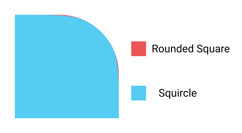
1.1. Comparison of a rounded square and quad circle: obviously, the difference is small

Industrial designers have long known how important rounding is for object perception. Look closely at the corners of the Macbook or at the old-style case for wired headphones under a desk lamp. Notice how difficult it is to find a position in which the corners throw sharply contrasting glare.

The reason is the continuity of rounding, which are specially designed by designers. It is not surprising that Apple, which has a unique experience in developing both software and hardware, ultimately applied the ideas of industrial design in the design of interfaces, making its icons look like physical things of their own production.

From form to formula

Of course, at Figma, we love iOS designers and we believe that our users should always have the right platform elements at hand. To give them access to this new form when designing, you need to find the exact mathematical description. Then we will begin to figure out how to embed this form in our tool.

Fortunately, people are asking this question since the release of iOS 7. Of course, we are not the first to follow this path! The original fundamental work of Mark Edwards contained a screenshot indicating that the shape of the icon is a special generalization of the ellipse called the superellipse. The following mathematical formula describes circles, ellipses, and superellipses, depending on the choice of a , b, and n :


2.1. Superellipse formula

Say, if you choose n = 2, a = 5 and b = 3, you get a normal ellipse with large semi-axes 5, oriented along the x axis, and small semi-axes 3, oriented along y . If we leave n = 2 and choose a = b = 1, then we get an ideal circle of unit radius. But if you choose n more than two, you get a super-ellipse - a rounded elliptical shape that begins to merge with the shape of the rectangle in which it is inscribed, where the angles become perfectly straight if n tends to infinity. Initially it was assumed that Apple chose a form with n = 5. If you try this formula , you will see that it is really very close to that used in iOS 7+.

If the true description were really so, then we could simply apply some reasonable number of Bezier curves — and then neatly integrate the new concept into Figma. But unfortunately, a careful subsequent analysis showed that the superellipse formula does not quite fit (although these days true superellipses are actually used as other icons). In fact, for all variants of n in the above equation there is a small but systematic discrepancy compared with the actual shape of the icon.

This is the first dead end in history: we have an elegant, simple equation for something very similar to the quad-circle iOS, but it is fundamentally wrong. But we must give our users the right equation.

Moving forward requires serious effort, and again I am happy to harvest the crops sown by others. One researcher, Mike Swanson of Juicy Bits, hypothesized that the angles of a quad circle are based on a sequence of Bezier curves. He applied a genetic algorithm to optimize the similarity with the official form of Apple. The results obtained correspond to the original, as proved by an excellent direct comparison of Manfred Schwind, who studied the iOS code that directly generates the icons. Thus, we have two different approaches that give the same structure of Bezier curves: the quad-circles of iOS 7 have been cracked and double-checked by independent researchers, and we don't even need to calculate anything!

File in action

Two important details remain that prevent us from cloning the form directly into Figma.

First, the surprising fact is that the version of the iOS formula (at least during the study) is made with some quirks - the corners are not quite symmetrical, but on the one hand there is a tiny straight segment that should not be here explicitly. We do not need it, because it complicates both the code and the tests, it is easy to remove it by simply mirroring half the corner where the bug is missing.

Secondly, when aligning the aspect ratio of a real rectangle from iOS, the shape of the icon changes dramatically from the quad circle we need to a completely different shape. Designers will be unpleasant such a quirk, and it makes it clear to determine what forms "should" manifest under certain conditions.

The most natural and useful behavior in the alignment of a quad circle would be the gradual disappearance of smoothing until there is no place for the transition between the round and straight parts of the angle. Further alignment should reduce the radius of the rounded section, which corresponds to the current Figma behavior. The Apple quad-circle formula here doesn’t help us much, because the rounding is done in a fixed way: it doesn’t give instructions on how to approach or move away from the old rectangle with rounded corners. What we really need is a parameterizable rounding, where a certain parameter value fits very closely with the shape of Apple.

As an additional bonus, if we can parameterize the transformation of a rectangle with rounded corners into a quad circle, then we can fully apply the same process in other places of Figma where rounding is used: stars, polygons and even corners in arbitrary hand-drawn vector networks. Despite the complexity, it starts to look much more complete and valuable than just adding the quad quad iOS 7. Now we give designers an infinite variety of new forms to use in many situations, and one of them corresponds to the icon of the quad circle with which it all started.

The requirement that our quad-circle rounding pattern be smoothly adjusted, but at the same time conforms to the shape of iOS 7 at a certain convenient point from the adjustment range - this is the first limitation in our history that has arisen and is difficult to satisfy. For a ballerina, a similar task would be to design a whole leap over one photo in flight, so that at a certain point the phase of the jump would correspond to the photo. Sounds damn hard. So maybe you still need some kind of calculation?

Powerful tool: differential geometry of flat curves

Before plunging into the parametrization of quad-circles, let’s step back and blow away the dust from some formal tools that will help us analyze what is happening. First of all, you need to decide how to describe a quadro-circle. Previously, in the case of superellipses, we used the equation with x and y , where all points ( x, y ) on the plane satisfying the conditions of the equation derived the superellipse. This is elegant in the case of a simple equation, but real quad-circles are a patchwork of connected Bezier curves, which leads to uncontrolled accumulation of equations.

We can cope with this complication using a more explicit approach: take one variable t , restrict it to a finite interval and compare each value of t in this interval with a separate point on the perimeter of the quad circle (in fact, Bezier curves are almost always represented in this way). If we concentrate only on one of the angles, thereby limiting our analysis to a curved line with a clear beginning and end, then we can choose such a mapping between t and an angle, so that t = 0 corresponds to the beginning of the line, t = 1 corresponds to the end of the line, and a smooth change in t from 0 to 1 smoothly traced the rounded portion of the corner. In mathematical language, we describe our angle of the curve r (t) , which is structured as


4.1. Bijection of a flat curve with [0,1]

where x (t) and y (t) are separate functions of t for the x and y components of r. We can imagine r (t) as a peculiar history of the path, say, of your trip by car. For each time point t between departure and arrival, you can estimate r (t) and get your car's position on the route. From the path r (t), we can derive the speed v (t) and the acceleration a (t) :


4.2. Speed ​​and acceleration of a flat curve

Finally, the mathematical curvature, which plays a major role in our history, in turn, can be expressed in terms of speed and acceleration:


4.3. Unsigned curvature of plane curves

But what does this formula really mean? Although it may look a bit complicated, the curvature has a simple geometric structure, originally due to Cauchy:

1. The center of curvature C at any point P along the curve lies at the intersection of the normal line to the curve in P and the other normal line taken infinitely close to P. (As a note, a circle centered in C is called an oscillating circle in P , from the Latin verb osculare , which means “kiss.” Isn't that wonderful?)
2. The radius of curvature R is the distance between C and P.
3. The curvature κ is the reciprocal of R.

As shown above, the curvature κ is non-negative and does not differ by turning it right or left. Since this difference is important to us, we form a κ sign curvature k , assigning a positive sign if the curve turns to the right, and a negative sign if to the left. This concept can also be compared with driving a car: at any point t, the sign curvature k (t) is simply the angle the steering wheel turns at time t , with a plus sign for turning right and minus for turning left.

Geometry taxis: parameterization of the arc length

With the introduction of curvature, only a few details remain to be settled. First, let's imagine for a moment two cars moving along the corner of a quad; one car accelerates sharply, and then it slows down all the time, while the other one evenly runs to the very end. These two different ways of driving will give rise to very different path histories, even with the same trajectory. We are concerned only with the shape of the corner, and not with the way to achieve it, so how can they lead to a common denominator? Here the main thing when marking the points of history is not to use time, but the cumulative distance traveled, that is, the length of the arc. That is, instead of asking the question “Where was the car ten minutes away?” It’s better to answer the question “Where was the car ten miles from the start of the trip?”. This way of describing the trajectory captures only the geometry and nothing more.

If we have some history of the path r (t) , we can always extract the arc length s as a function of the time t of the path, integrating the speed as follows:


5.1. Arc length integral

If we can invert this relation and find t (s) , then we can substitute it in place of t in our history for the path r (t) to get the desired parametrization of the arc length r (s) . Parameterization of the arc length for a path is equivalent to the history of the path of a car moving at unit speed, so it is not surprising that the speed v (s) is always the unit vector and the acceleration a (s) is always perpendicular to the speed. Consequently, in the variant with parametrization along the arc length, the description of the curvature is simplified only to the magnitude of the acceleration.


5.2. Curvature in option with parameterization by arc length

And you can set the corresponding right or left character to form the signed curvature k (s) . Obviously, most of the complications in the more general definition of curvature were simply the non-geometric content of the path history. In the end, the curvature is a purely geometric quantity, so it is very nice to see that it looks simple in geometrical parametrization.

Design the curvature, calculate the curve

Now for another detail. We have just figured out how to go from describing the history of the path r (t) to the description by the arc length parameter r (s) and how to extract the sign curvature k (s) from it. But can we do the opposite? Design a curvature profile - and draw a parent curve from it? Let's look again at the analogy with the car: suppose that when we were driving at a constant unit speed throughout the route, we fixed the position of the steering wheel continuously throughout the journey. If we take this steering data and then transfer it to another driver, will he be able to fully restore the route, if he correctly reproduces the steering wheel positions and drives at exactly the same speed? Intuitively, we have enough information to restore the parental curve, but how does this calculation look mathematically? Although a bit rough, but this is possible thanks to Euler through the parameterization of the arc length. If we choose such a coordinate system so that the curve starts at the origin and is initially directed along the x axis, then x (s) and y (s) can be reconstructed from k (s) as follows:


6.1. Recovery of a curve by its curvature

Finally, notice the argument of the sine and cosine functions: this is the integral of the sign curvature. Usually, trigonometric functions specify angles in radians as arguments. So it is in our case: the integral from a to b is the signed curvature - this is the course in b minus the course in a . Thus, if you take a rectangle and round the corner as you please, measure the curvature of the rounded part and integrate the result, in the end we will always get π / 2 .

Quadro Circle Anatomy

Having dealt with the details, apply these analytical tools to some real forms. Let's start with the rounded corner of the rectangle, with the radius of the angle equal to one. First we construct the angle itself, and then the curvature as a function of the arc length:


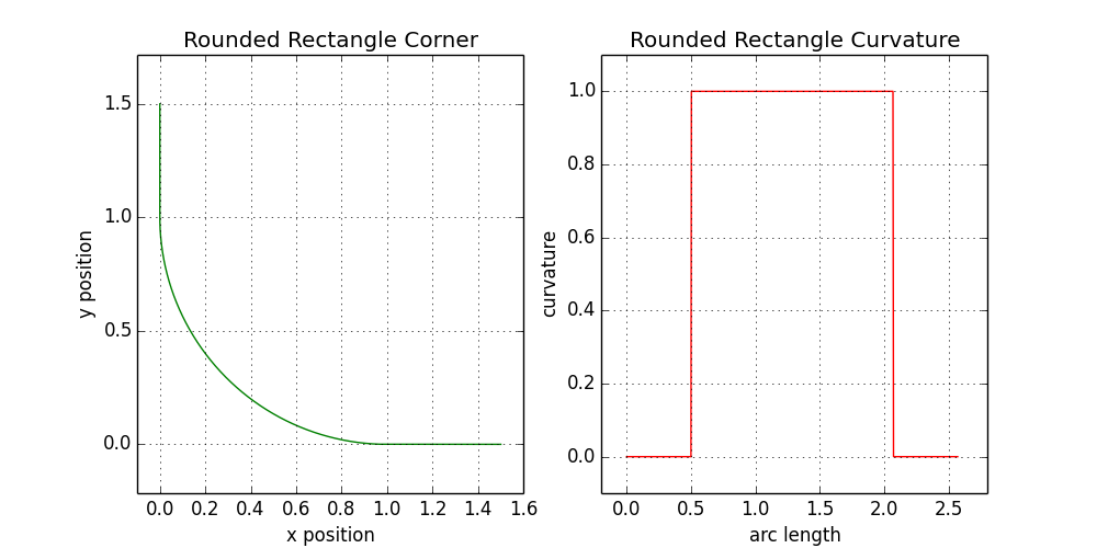
7.1. Curvature Analysis of a Rounded Rectangle

Now we repeat the process for the corners of real Apple quadro circles — and see that their curvature is very different:


7.2. Analysis of the curvature of the quad-circle iOS 7

The curvature looks quite jagged, but this is not necessarily bad. As we will see later, you can find a compromise between a smooth curve of curvature and a small number of Bezier curves, and there are only three in the corner of iOS. As a rule, designers are ready to sacrifice a mathematically perfect curvature profile for the sake of reducing the number of Bezier curves. Discarding the details, the overall picture appears on the right graph: the curvature rises, aligns in the middle, and then returns down.

Breakthrough: Parameterized Smoothing

Bingo! In this last observation lies the key to how to parametrize the smoothing angle of our quad circle. With zero smoothing, the curvature profile will look like a rounded rectangle: in the form of a tabletop. As the smoothing gradually increases, the height of the tabletop remains unchanged, but its edges turn into steep slopes, forming an isosceles trapezoid profile (of course, still with a common π / 2 angle). When smoothing approaches a maximum, the flat part of the trapezoid disappears - and we get a wide isosceles triangle, whose height corresponds to the height of the original table top.


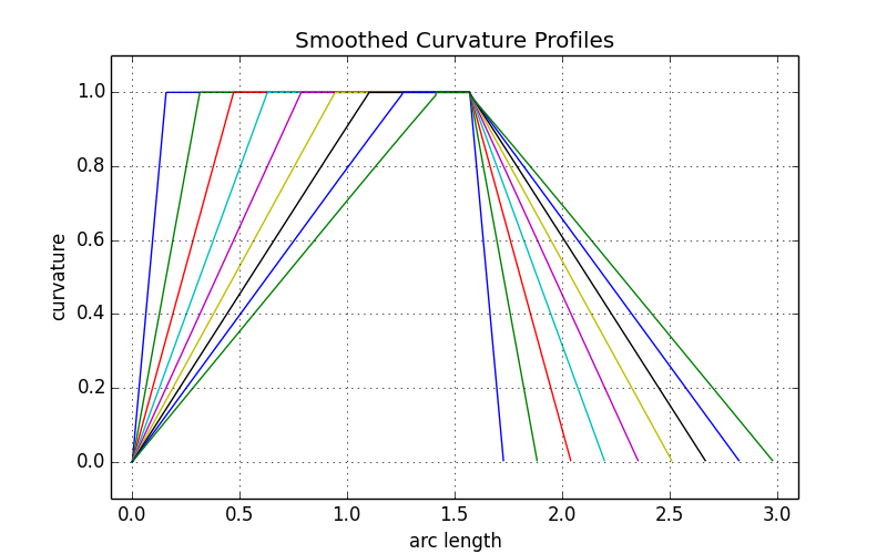
8.1. Curvature profiles for different values ​​of the smoothing parameter

Let us try to express this sketch of the curvature profile in mathematical terms, using ξ as the smoothing parameter, which varies from zero to one. To provide for use with other forms where there are no right angles, we will also introduce a rotation angle θ , which in the case of a rectangle is π / 2 . Combining them together, we can express a piecewise continuous function in three parts: one for lifting curvature, one for a flat top, and a third for descending:


8.2. Parameterization of the curvature profile of a quad

Note that the first and third parts (ascent and descent) disappear when ξ approaches zero, and the middle part (flat top) disappears when ξ approaches unity. Above, we have shown how to go from the curvature profile to the parent curve. Let's try to do this on the first equation, which describes a line whose curvature starts from zero and increases steadily. First, we make a simple inner integral:


8.2. The first integral of 6.1 as applied to equations 8.2

So far, everything is fine! You can continue and form the following pair of integrals:


8.2. The second integral of 6.1 as applied to equations 8.2 (Fresnel integral)

Alas, here we are stuck, because these integrals are not so simple. If you have heard about the connection between trigonometric functions and exponents, you can guess that these integrals are related to the error function, which cannot be expressed by elementary functions. The same applies to these integrals. So what are we going to do? The solution is beyond the scope of this article (see this post on Math StackExchange for a hint), but in this case, you can replace the sine and cosine in power series, and then change the sum and integral:


8.4. Fresnel integral expansion

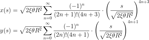
Power series seems almost impassable, so let's take another step and explicitly write down the first few elements in each row, multiplying everything to simplify. This gives the following several elements for the x and y forms:


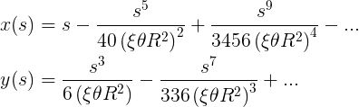
8.5. Low order elements (n <3) of 8.3

Apotheosis of clothoid

This is a specific result! We can actually draw a graph of this pair of equations (with a reasonable choice of ξ , θ and R ) - and get the contour as a function of s . If we had an arbitrary number of elements and the ability to calculate sums, we would see that as s increases, the curve twists into a spiral, although this happens far from the area of ​​interest.

Repeating the thesis from the beginning of this article, we are again not the first to engage in such research. Due to the linear curvature, which is very useful in practice, many have stumbled upon this curve in the past. It is known as the Euler Spiral, the Cornu Spiral or Clothoid - and is widely used in the design of tracks, including highways and roller coasters.


9.1. Clothoid to s = 5

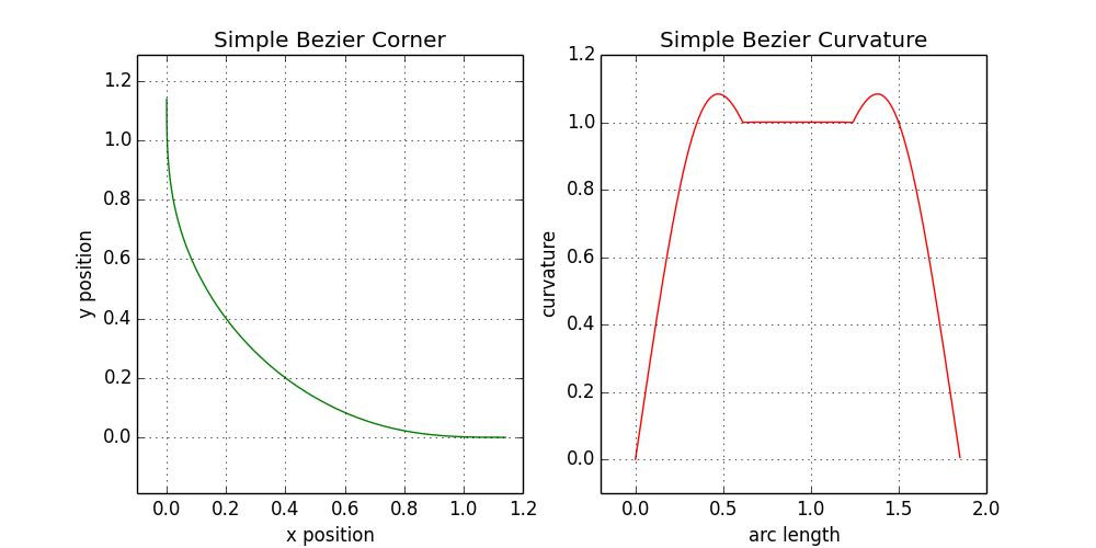
If we use the decomposition only to n <10, as indicated in 8.5, then we finally have everything we need to produce the first artifact. This series is the ascending (first) part of equation 8.2, but it is easy to adapt to the descending (third) part, and we will link these parts together with an arc segment for the flat (second) part. Such a method provides a mathematically perfect angle of a quad circle, which exactly corresponds to the curvature construction, first presented in equations 8.2. , ξ = 0,4:


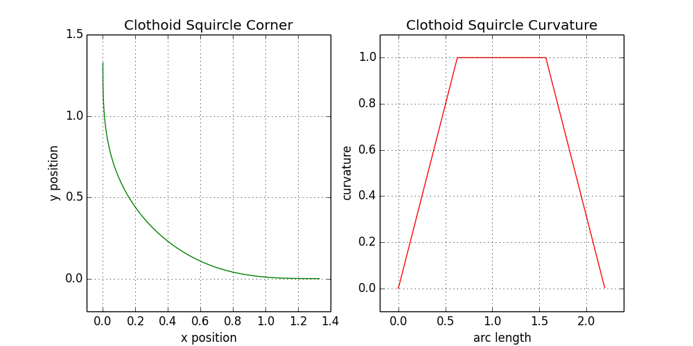
9.2. ξ = 0,4

, , . . , ξ — .

, s . Figma ( — ). . x(s) y(s) . , .

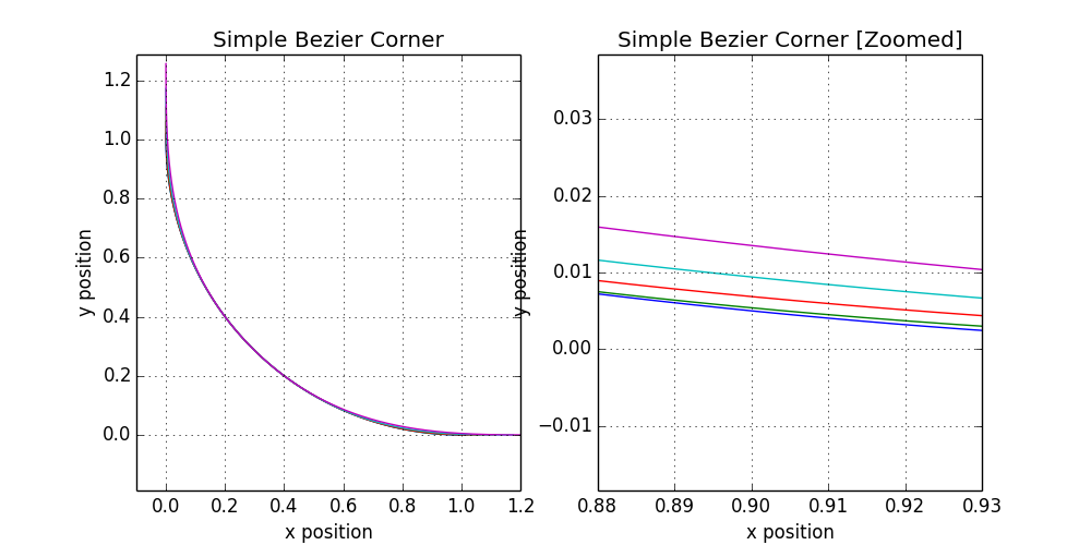
, , ξ . ξ = 0,9:


9.3. ξ = 0,9

. , , . , , ( ). , , . .

, — , .

-, , , , ξ . , UI c . , . , . , iOS , , ξ . , , ξ .

-, , . Apple ( ) , — , ?

Thirdly, we have some incomprehensible technical limitations. They are not obvious from the very beginning, but become a serious problem of implementation. To understand them, consider a square of 100 × 100 pixels, with a standard rounding for a corner radius of 20px. This means that on each side of the square, 60px of straight segment remains. If we flatten a square into a 80 × 100px rectangle, then the straight section of the short side will be only 40px. What happens when we narrow the rectangle so much that we end with a straight fragment? Or if we continue to narrow it further into a rectangle, say, 20 × 100px? At the moment, Figma determines the maximum applicable value of the rounding of corners - and uses it. Thus, in a 20 × 100px rectangle there will be a rounding with a radius of 10px.

R ξ p , p(R,ξ) ξ(R,p).

, . 100×100px, 20px, , 12 . 36px . 60×100px? , , . ξ , ? , .

, : Rand the parameter ξ consumes p pixels, then the function p (R, ξ) must be reversible in ξ (R, p) . This is a somewhat hidden limitation, which also excludes a solution of a high order nearby clothoid.

Finally, we have a limit of usability: the change in smoothing should be at least somehow noticeable in the figure. If we pull the smoothing parameter ξ back and forth between zero and one, we would like to see the difference! Imagine that all our work leads only to barely noticeable changes - this is unacceptable. This is essentially a requirement of utility, and in fact this is the most important limitation.

The simpler the better

, , . , . .


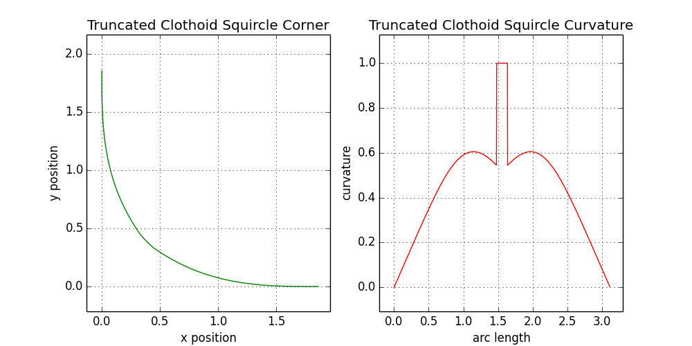
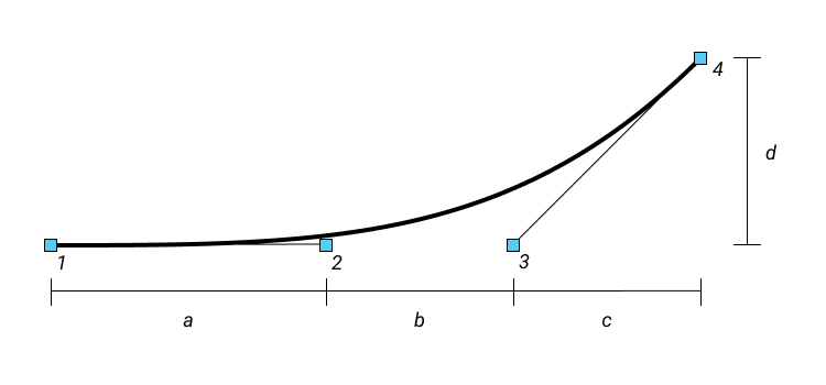
11.1.

. -, 1, 2 3 . 1, . , 1 P1 , 2 P2 .., 1 :


11.2. Unsimplified curvature at point 1 in Fig. 11.1.

Reduction of a fraction is clearly visible if points 1–3 are lined up. We apply the same formula to point 4, indicating the coordinates in the reverse order:


11.3. The simplified curvature at point 4 in Fig. 11.1

Ideally, the curvature will be the same as in the circular section, or 1 / R , which leads to another constraint. Finally, the values ​​of c and d are fixed because of the fact that the end of this curve must coincide with the circular part and touch the points of contact. Therefore, the above curvature constraint simply gives us the value of b :


11.4. Solution for b in fig. 11.1, ensuring continuity of curvature

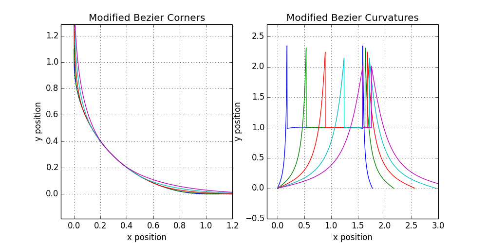
( 1), a b , . , , ξ = 0,6.



, . , ξ 0 1 . , ξ = 0,1, 0,3, 0,5, 0,7 0,9 :



Despite the good mathematical properties, the effect is barely noticeable. Of course, this option is closer to the real product than the curve obtained earlier by reducing the number of clothoid. If only to customize the formula for greater variability!

Small touches

, . , , , ξ . . , , .

- , . , θ , R , q , q :


12.1.

p(R,ξ) q , :


12.2.

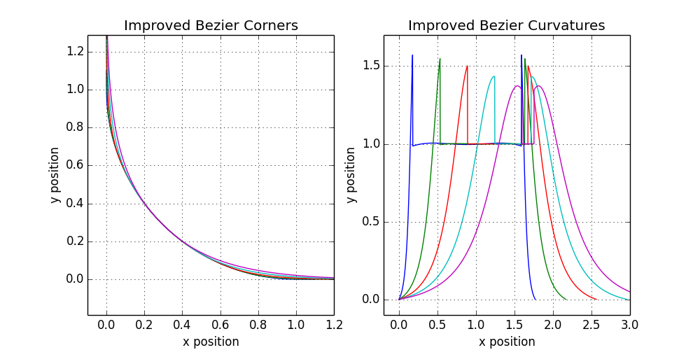
, , . a + b . , c d , a + b , : a b ? , , a = bthen we will finish with the definition of the parametrization of a Bezier curve, the angles and curvatures of which are shown below:


12.3. The shape of the angle and the curvature profile for a simple smoothing scheme

Such a visual variety already looks promising! Curves look attractive and whole. But the curvature profile is coarse. Now, if a little smooth peaks, then you get a serious candidate for the final release. Despite the weak profile, even in this simple family of forms there is an instance, very similar to the version of Apple’s quad circle. It is almost good enough to roll it out for our users with a clear conscience.

We now turn to the curvature profile, our last unsolved problem. Instead of evenly dividing the difference between a and b , , a, b ? , . :


12.4.

, - . ξ = 0,6 iOS, . : ? Nothing.

As a result, it is useful to reflect on the process itself. This story has repeatedly confirmed the same thing - the strength and effectiveness of the simplest possible approach. In the worst case, we will get a base for comparison, if it does not work. His serious assessment will help determine the most important things that should be considered when finalizing the approach and further progress. And at best, like ours, the simplest approach already gives a fairly good result!

In the end, I want to reflect on the difference between a good and a perfect product. I'm a little embarrassed that I did not come up with a better curvature profile. I am sure that it was possible to allocate more time, because there are many options for research. From an intellectual point of view, it is a bit unpleasant that we received such a beautiful series of clothoid, but could not use it in the final version. But there is a more important conclusion: the time constraints when working in a small company are very real - and the design that violates them cannot be considered good.