Tutorial: toon-contours in Unreal Engine 4

When talking about "toon-contours", they mean any technique that renders lines around objects. Like cel shading, the outlines help the game look more stylized. They can create the feeling that objects are painted or inked. Examples of this style can be seen in games such as Okami , Borderlands and Dragon Ball FighterZ .

In this tutorial you will learn the following:

• Create outlines using an inverted mesh
• Create paths using post processing and convolutions
• Create and use material functions
• Sampling adjacent pixels

Note: this tutorial assumes that you already know the basics of the Unreal Engine. If you are new to the Unreal Engine, then I recommend to explore my series of tutorials from ten parts of the Unreal Engine for beginners .
')
If you are not familiar with the post-processing of materials, then you should first study my cel shading tutorial. In this article we will use some of the concepts described in the cel shading tutorial.

Getting Started

To get started, download materials from this tutorial. Unzip them, go to ToonOutlineStarter and open ToonOutline.uproject . You will see the following scene:


First we create the outlines using an inverted mesh .

Inverted Mesh Contours

The principle of implementing this method is to duplicate the target mesh. Then the duplicate is assigned a solid color (usually black) and its size is increased so that it is slightly larger than the original mesh. So we will create a silhouette.


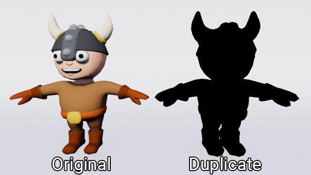
If you use just a duplicate, it will completely block the source mesh.


To fix this, we can invert the duplicate normals. When the backface culling parameter is on, we will see not the outer, but the inner edges.


This will allow the source mesh to shine through the duplicate. And since the duplicate is larger than the original mesh, we get the outline.


Benefits:

• You will always have clear lines, since the contour consists of polygons.
• The appearance and thickness of the contour is easy to adjust by moving the vertices
• With distance, the contours become smaller (this may be a disadvantage).

Disadvantages:

• Usually, you cannot create contours of parts inside the mesh in this way.
• Since the contour consists of polygons, they are prone to clipping. This can be seen in the example above, where the duplicate intersects with the ground.
• With this method, speed reduction is possible. It depends on how many polygons are in the mesh. Since we use duplicates, we essentially double the number of polygons.
• Such contours better manifest themselves on smooth and convex meshes. Sharp edges and concave areas will create holes in the contour. This can be seen in the image below.

Creating an inverted mesh is better in a 3D modeling program, this gives more control over the silhouette. When working with skeletal meshes, this also allows skin duplication of the duplicate with the original skeleton. Due to this, the duplicate will be able to move along with the original mesh.

For this tutorial, we will create a mesh not in a 3D editor. and in Unreal. The method is slightly different, but the concept remains the same.

First we need to create a duplicate material.

Creating Inverted Mesh Material

For this method, we will mask the polygons with the faces out, and as a result we will have polygons with the faces inwards.

Note: due to masking, this method is a bit more expensive than manually creating a mesh.

Navigate to the Materials folder and open M_Inverted . Then go to the Details panel and change the following parameters:

• Blend Mode : select Masked for it. This will allow us to mark areas as visible or invisible. The threshold value can be changed by editing the Opacity Mask Clip Value .
• Shading Model: select the Unlit value. Due to this, the mesh will not be affected by the lighting.
• Two Sided: select the value enabled . By default, Unreal cuts back edges. Turning on this option disables the clipping of the rear edges. If you leave clipping of the back edges turned on, then we will not be able to see the polygons with the faces inside.

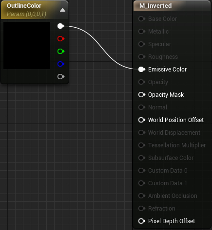
Next, create a Vector Parameter and name it OutlineColor . It will control the color of the contour. Connect it with Emissive Color .


To mask out polygons, create TwoSidedSign and multiply it by -1 . Attach the result with the Opacity Mask .


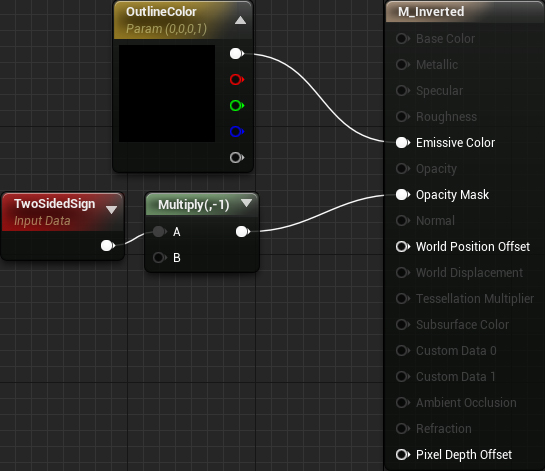
TwoSidedSign displays 1 for the front faces and -1 for the back faces. This means that the front faces will be visible, while the rear faces will be invisible. However, we need the opposite effect. To do this, we change the signs by multiplying by -1 . Now the front faces will give -1 at the output, and the rear ones 1 .

Finally, we need a way to control the thickness of the contour. To do this, add the selected nodes:


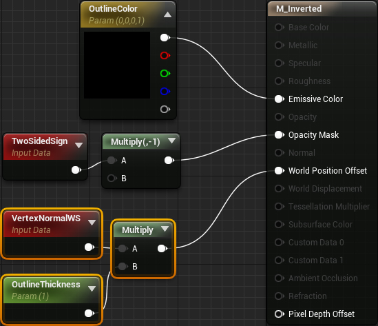
In the Unreal engine, we can change the position of each vertex using World Position Offset . By multiplying the vertex normal by OutlineThickness , we make the mesh thicker. Here is a demo using the original mesh:


At this point we finished preparing the material. Click Apply and close M_Inverted .

Now we need to duplicate the mesh and apply the newly created material.

Duplicate mesh

Go to the Blueprints folder and open BP_Viking . Add the Static Mesh component as a Mesh child and name it Outline .


Select Outline and select SM_Viking for Static Mesh . Then select MI_Inverted for its material .


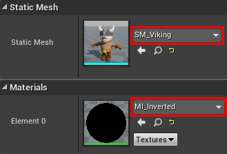
MI_Inverted is an instance of M_Inverted . It will allow us to change the OutlineColor and OutlineThickness parameters without recompiling.

Click on Compile and close BP_Viking . Now the viking will have an outline. We can change the color and thickness of the contour by opening MI_Inverted and adjusting its parameters.


And on this we are done with this way! Try to create an inverted mesh in a 3D editor and then transfer it to Unreal.

If you want to create contours differently, you can use post-processing for this.

Creating contours by post processing

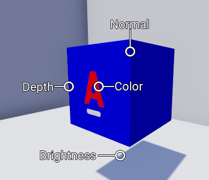
You can create post-processing contours using edge recognition . This is a technique that recognizes breaks in image areas. Here are some types of breaks you can look for:


Benefits:

• The method is easily applicable to the whole scene.
• Constant computational cost, since the shader is always executed for each pixel.
• The thickness of the line always remains the same regardless of the distance (this may be a disadvantage).
• Lines are not clipped by geometry, since this is a post-processing effect.

Disadvantages:

• Usually for recognition of all edges it is required several edge recognizers. This reduces speed.
• The method is subject to noise. This means that the edges will appear in areas where there is great variation.

Usually, edge recognition is performed by convolving each pixel.

What is a "convolution"?

In the image processing area, convolution is an operation on two groups of numbers to calculate a single number. First we take a grid of numbers (known as the core ) and position the center above each pixel. Below is an example of how the kernel moves over two lines of an image:


For each pixel, each element of the core is multiplied by the corresponding pixel. To demonstrate this, let's take a pixel from the upper left edge of the mouth. Also, to simplify the calculations, we convert the image to grayscale.


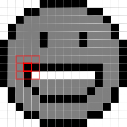
First, we locate the core (we take the same one that was used above) so that the target pixel is in the center. Then multiply each element of the core by the pixel on which it is superimposed.


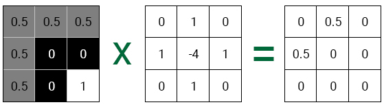
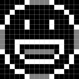
Finally, add the results together. This will be the new value for the center pixel. In our case, the new value is 0.5 + 0.5 or 1 . Here is what the image looks like after performing a convolution for each pixel:


The resulting effect depends on the core used. The kernel from the examples shown above is used to recognize edges. Here are some examples of other edges:


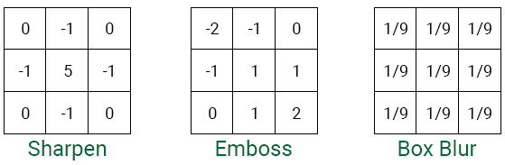
Note: You may notice that they are used as filters in image editors. In fact, many operations with filters in image editors are performed using convolutions. In Photoshop, you can even perform convolutions based on your own kernels!

To recognize the edges of the image, you can use Laplace edge recognition.

Laplace edge recognition

First, what will be the core for Laplace edge recognition? In fact, we have already seen this core in the examples of the previous section!


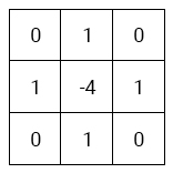
This core performs edge recognition because the Laplacian measures changes in steepness. Areas with large variations deviate from zero and report that this is an edge.

To understand this, let's look at the Laplacian in one dimension. The core for it will be as follows:


First position the core above the edge pixel, and then perform the convolution.


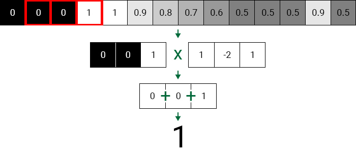
This will give us a value of 1 , which indicates that there has been a big change. That is, the target pixel is likely to be an edge.

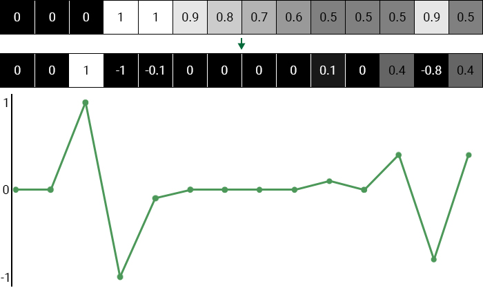
Next, let's perform a convolution of a region with less variability.


Even though the pixels have different values, the gradient is linear. That is, there is no change in slope and the target pixel is not an edge.

Below is the image after convolution and a graph of all values. You can see that the pixels on the edge more strongly deviate from zero.


Yes, we considered quite a lot of theory, but do not worry - now the interesting begins. In the next section, we will create a post-processing material that will perform Laplace edge recognition in the depth buffer.

Build a Laplace Rib Detector

Go to the Maps folder and open PostProcess . You will see a black screen. This happened because the map contains Post Process Volume, which uses blank post-processing material.


It is this material that we will modify to build the edge recognizer. The first step is that we need to figure out how to sample the adjacent pixels.

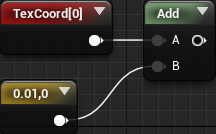
To get the position of the current pixel, we can use TextureCoordinate . For example, if the current pixel is in the middle, it will return (0.5, 0.5) . This two component vector is called UV .


To sample another pixel, we just need to add an offset to TextureCoordinate. In an image of 100 × 100, each pixel in the UV space has a size of 0.01 . To sample the pixel on the right, add 0.01 along the X axis .


However, there is a problem here. When the image resolution changes, the pixel size also changes. If we use the same offset (0.01, 0) for the image 200 × 200, then two pixels will be sampled on the right.

To fix this, we can use the SceneTexelSize node, which returns the pixel size. To apply it, you need to do something like this:


Since we are going to sample several pixels, we need to create it several times.


Obviously, the graph will quickly become confused. Fortunately, we can use the functions of the materials to keep the graph legible.

Note: The material function is similar to the functions used in Blueprints or in C ++.

In the next section, we will insert duplicate nodes into the function and create an input for the offset.

Create pixel sampling function

To get started, go to the Materials \ PostProcess folder . To create a material function, click on Add New and select Materials & Textures \ Material Function .


Rename it to MF_GetPixelDepth and open it. There will be one FunctionOutput node in the graph. This is where we will append the value of the sample pixel.


First we need to create an input that will receive an offset. To do this, create a FunctionInput .


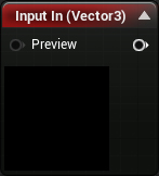
When we continue to use the function, it will be the input contact.

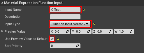
Now we need to set several parameters for the input. Select FunctionInput and go to the Details panel. Change the following parameters:

• InputName: Offset
• InputType: Function Input Vector 2. Since the depth buffer is a 2D image, the offset must be of type Vector 2 .
• Use Preview Value as Default: Enabled. If you do not pass the input value, the function will use the value from the Preview Value .

Next, we need to multiply the offset by the pixel size. Then you need to add the result to TextureCoordinate. To do this, add the selected nodes:


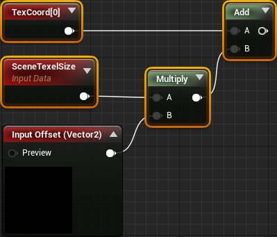
Finally, we need to sample using a UV depth buffer. Add SceneDepth and connect everything as follows:

Note: You can also use SceneTexture instead with a SceneDepth value.

Summarize:

1. Offset gets Vector 2 and multiplies it by SceneTexelSize . This gives us a shift in UV space.
2. Add an offset to TextureCoordinate to get a pixel located (x, y) pixels from the current one.
3. SceneDepth will use the transmitted UVs to sample the corresponding pixel, and then output it.

And on this work with the function of the material is finished. Click on Apply and close MF_GetPixelDepth .

Note: You can see an error in the Stats panel telling you that only translucent or post-processing materials can read from the back of the scene. You can safely ignore this error. Since we will use the function in the post-processing material, everything will work.

Next we need to use the function to perform the convolution of the depth buffer.

Convolution

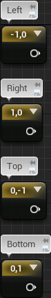
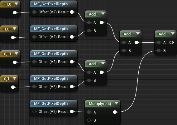
First we need to create offsets for each pixel. Since the corners of the core are always zero, we can skip them. That is, we have left, right, upper and lower pixels.

Open PP_Outline and create four Constant2Vector nodes. Give them the following parameters:

• (-ten)
• (ten)
• (0, -1)
• (0, 1)

Next we need to sample five pixels in the core. Create five MaterialFunctionCall nodes and select MF_GetPixelDepth for each. Then connect each offset with its own function.


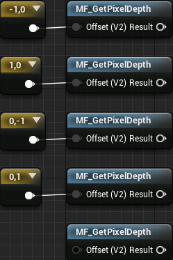
So we get the depth values ​​for each pixel.

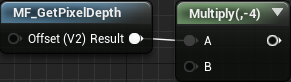
The next step is the multiplication stage. Since the multiplier for neighboring pixels is 1 , we can skip the multiplication. However, we still need to multiply the central pixel (lower function) by -4 .


Next, we need to summarize all the values. Create four Add nodes and connect them as follows:


If you remember a plot of pixel values, you will notice that some of them are negative. If you use the material as it is, negative pixels will appear black, because they are less than zero. To fix this, we can get an absolute value that converts all input data to a positive value. Add Abs and mix it up like this:


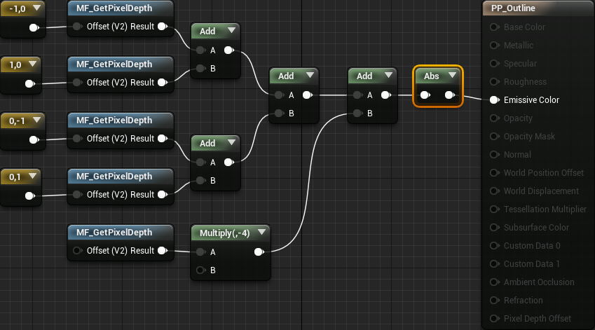
Summarize:

1. MF_GetPixelDepth nodes get the depth value from the center, left, right, top and bottom pixels.
2. Multiply each pixel by its corresponding core value. In our case, it is enough to multiply only the central pixel.
3. Calculate the sum of all pixels.
4. We get the absolute value of the amount. This will not allow pixels with negative values ​​to appear in black.

Click on Apply and return to the main editor. All lines now appear on the image!


However, here we have some problems. First, there are edges in which the difference in depth is insignificant. Secondly, there are circular lines against the background, because it is a sphere. This is not a problem if you limit the recognition of the edges only meshes. However, if you want to create lines in the whole scene, then these circles are undesirable.

To correct this, you can use threshold values.

Implementation thresholds

First we correct the lines that appear due to minor differences in depths. Return to the material editor and create the diagram shown below. Set Threshold to 4 .


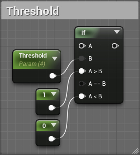
Later we connect the edge recognition result with A. It will output a value of 1 (indicating an edge) if the pixel value is higher than 4 . Otherwise, it will output 0 (no edge).

Next we get rid of the lines in the background. Create the schema shown below. Set the DepthCutoff value to 9000 .


In this case, the output will be transferred to the value 0 (no edge), if the depth of the current pixel is more than 9000 . Otherwise, the value from A <B will be transmitted to the output.

Finally, connect everything as follows:


Now the lines will be displayed only when the pixel value is greater than 4 ( Threshold ) and its depth is less than 9000 ( DepthCutoff ).

Click on Apply and return to the main editor. Small lines and lines in the background is no more!

Note: You can create an instance of PP_Outline material to control Threshold and DepthCutoff .

Edge recognition works quite well. But what if we need thicker lines? For this we need to increase the size of the kernel.

Creating thicker lines

In general, the larger the kernel size, the more it affects the speed, because we need to sample more pixels. But is there a way to enlarge the cores while maintaining the same speed as with a 3 × 3 core? This is where the extended convolution comes in handy.

With an expanded convolution, we simply spread the offsets further. To do this, we multiply each offset by a scalar, called the coefficient of expansion . It determines the distance between the elements of the core.


As you can see, this allows us to increase the size of the core, while sampling the same number of pixels.

Now let's implement the extended convolution. Return to the material editor and create a ScalarParameter called DilationRate . Set it to 3 . Then multiply each offset by DilationRate .


So we will shift each offset a distance of 3 pixels from the central pixel.

Click on Apply and return to the main editor. You will see that the lines are much thicker. Here is a comparison of lines with different expansion factors:


If you are not making a line-style game, then most likely you need the original scene to be visible. In the last section, we will add lines to the image of the original scene.

Adding lines to the original image

Return to the material editor and create the diagram shown below. Order is important here!


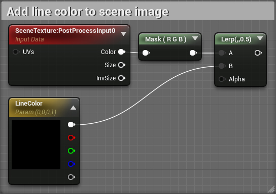
Next, connect everything as follows:


Now Lerp will display the image of the scene if alpha reaches zero (black color). Otherwise, it displays LineColor .

Click on Apply and close PP_Outline . Now the original scene has contours!

Where to go next?

The finished project can be downloaded here .

If you want to work with edge recognition, try creating a recognition that works with the normal buffer. This will give you some edges that do not appear in the edge resolver by depth. Then you can combine both types of edge recognition together.

Convolutions is an extensive topic that finds active use, including in artificial intelligence and sound processing. I recommend to study the convolutions, creating other effects, such as sharpening and blurring. For some of them, simply changing the kernel values ​​is enough! See an interactive explanation of the bundles in Images Kernels explained visually . It also describes the kernel for some other effects.

I also strongly recommend to watch the presentation with GDC on the Guilty Gear Xrd graphic style . For external lines, this game also uses an inverted mesh method. However, for internal lines, developers have created a simple, but ingenious technique using textures and UV.