Introducing Google's S2 Geo-Library and Case Studies
Hi, Habr!
My name is Marco, I work in Badoo on the Platform team. Not so long ago, on GopherCon Russia 2018, I told you how to work with coordinates. For those who do not like to watch the video (and of all those interested, of course), I publish a text version of my report.
')
Now most people in the world have a smartphone with constant access to the Internet. Speaking in numbers, in 2018 almost 5 billion people will have a smartphone, and 60% of them use the mobile Internet.
These are huge numbers. It became easy and simple for companies to receive user coordinates. These ease and accessibility have spawned (and continue to spawn) a huge number of services based on coordinates.
We all know companies like Uber , games that have conquered the world, such as Ingress and Pokemon Go . But what is there, in any banking application, you can see ATMs or discounts nearby.
We at Badoo are also very active in using coordinates to provide our users with the best, relevant and interesting service for them. But what kind of use are we talking about? Let's look at examples of services that we have.
Badoo is first of all dating. A place where people get to know each other. One of the important criteria when searching for people is the distance. Indeed, in most cases, a girl from Moscow wants to meet a boy who is a couple of kilometers away from her, or at least also lives in Moscow, and not in far Vladivostok.

Services that pick you people for a “yes / no game” or show users around are searching for people with the criteria that are appropriate for you within a certain radius of you.
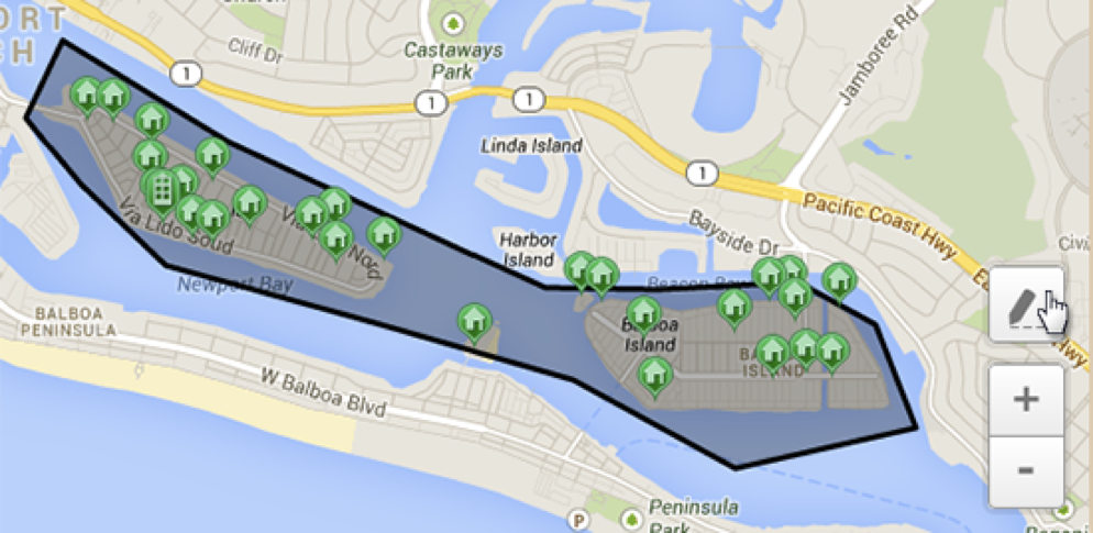
In order to answer the questions in which city the user is located, in which country or, more precisely, for example, at which airport or at which university, we use the Geoborder service, which deals with the so-called geofencing .

The easiest way to answer these questions would be to consider the distance from the user to the city center or the center of the university, but this approach is very inaccurate and depends on a large number of boundary conditions.
Therefore, we have drawn very precise borders of countries, cities, important objects (for example, universities and airports, of which I spoke). These borders are defined by polygons. Having a set of such boundaries, we can understand whether the user is inside a polygon, or find the nearest polygon to it. Accordingly, we can tell in which city he is, or find the city nearest to him.

We have a very popular feature called Bumped Into, which in the background constantly searches for users to intersect in time and space and shows you that you regularly visit the same place at the same time with this boy or this girl walk regularly the same way. This feature is very popular with users, because it is another reason to get acquainted with the topic with which you can start a conversation.
Well, the last example I’ll mention is related to caching geo-information. Imagine that you are using data from, for example, Booking.com, which provides you with information about hotels around, but to go to Booking.com every time is too long. Your internet pipe is probably quite narrow, like the pit of this gopher. Perhaps the service you go to for data takes money for each request and you want to save a little.

In this case, it would be nice to have a caching layer, which significantly reduces the number of requests to a slow or expensive service, and will provide a very similar API to the outside. A service that will understand that he already knows about all or most of the hotels in a given area, these data are relatively fresh, and, accordingly, you can not get behind them in an external service. Such tasks are solved in our service called Geocache.
We have already understood that there are a lot of coordinates, coordinates are important, and on the basis of them you can make a lot of interesting services. So what's next? What is actually the matter? How do the coordinates differ from any other information received from the user?
And I would say two features.

First, the geo-data is three-dimensional, or rather two-dimensional, because in the general case we are not interested in height. They consist of latitude and longitude, and the search most often goes simultaneously on both. Imagine searching in any area. Standard indexes in common DBMSs are not optimal for this use.
Secondly, many tasks require more complex data types such as polygons, which we discussed above using the example of the Geoborder service in Badoo. Polygons, of course, are composed of vertex coordinates, but require additional processing, and search queries for such data types are also more complicated. We have already seen the query "Find the nearest polygon to a point" or "Find a polygon that includes this point."
In order to comply with these features, many DBMSs include special indexes, sharpened for multidimensional data, and additional functions that allow you to work with objects such as polygons or broken lines.

Probably the most striking example is PostGIS - an extension to the popular PostgreSQL DBMS, which has the most extensive capabilities for working with coordinates and geography.
But using a ready-made DBMS is not the only and not always the best solution.

If you do not want to divide the business logic of your service between it and the DBMS, if you want something that is not available in the DBMS, if you want to fully manage your service and not be limited to scaling any DBMS, for example, then you can want to embed the ability to search and work with geo-data in your service.
Such an approach is undoubtedly more flexible, but it can be much more complicated, because the DBMS is an all-in-one solution, and many infrastructure-type replications are already done for you. Replications and, in fact, algorithms and indices for working with coordinates.
But not so scary. I would like to introduce you to the library, which implements most of what you need. Which is a kind of cube, easily embedded wherever you need to work with the geometry on the sphere or search by coordinates. With a library called S2 .
S2 is a library for working with geometry (including on a sphere), which provides very convenient possibilities for creating geo-indices.
Until recently, S2 was virtually unknown and had very poor documentation, but not so long ago, Google decided to " re-release " it in open-source, adding to the layout with a promise to support and develop the product.
The main version of the library is written in C ++ and has several official ports or versions in other languages, including the Go version. The go-version today is not 100% realizing everything that is in the C ++ version, but what is there is enough to implement most things.
In addition to Google, the library is actively used in companies such as Foursquare , Uber , Yelp , and of course Badoo . And among the products that use the library inside, you can highlight the well-known MongoDB.
But so far I have not said anything sensible about why S2 is convenient and why it makes it easy to write services with a geo search. Let me fix and immerse myself a bit in the guts before we look at two examples.

Usually geography involves the use of one of the most common projections of the globe on a plane. For example, we all know the projection of the Mercator . The disadvantage of this approach is that any projection somehow has distortions. Our globe with you is not very much like a plane.

Recall the famous picture with a comparison of Russia and Africa. On the maps, Russia is huge, and in fact, the area of Africa is already twice the area of Russia! This is just an example of the distortion of the Mercator projection.

S2 solves this problem by using exclusively spherical projection and spherical geometry. Of course, the Earth is also not quite a sphere, but distortions in the case of a sphere can be neglected for most tasks.
We will work with a unit, or unit-sphere , that is, with a sphere of radius 1 and we will use such concepts as the central angle , the spherical rectangle and the spherical segment .
The name S2 is derived from the mathematical notation denoting the unit sphere.
But you should not be afraid, as the library takes on almost all the mathematics.
The second (and most important) feature of the library is the concept of hierarchical partitioning of the globe into cells (in English - cells).
The division is hierarchical, that is, there is such a thing as a level (or level) of a cell. And at one level, the cells are about the same size.
Cells can set any point on Earth. If you use a cell of the maximum, 30th level, which is smaller than a centimeter in width, then the accuracy, as you understand, will be very high. The lower level cells can set the same point, but the accuracy will be less. For example, 5 m by 5 m.
Cells can be set not only points, but also more complex objects such as polygons and some areas (in the picture you, for example, see Hawaii). In this case, such figures will be given by sets of cells (possibly at different levels).
Such a partition is very compact: each cell can be encoded with one 64-bit number.
I mentioned that the cell is defined by one 64-bit number. Here it is! It turns out that a coordinate or a point on Earth, which by default is given by two coordinates, with which we are inconvenient to work with standard methods, can be given with a single number. But how to achieve this? Let's get a look…
How does the hierarchical division of the sphere occur?

We first surround the sphere with a cube and project it onto all six of its faces, slightly modifying the projection on the move to remove distortion. This is level 0. Then we can divide each of the six faces of the cube into four equal parts - this is level 1. And each of the four parts that we can get can be further divided into four equal parts - level 2. And so on until level 30.
But at this stage, we still have two-dimensionality. And here we come to the aid of a mathematical idea from the distant past. At the end of the 19th century, David Hilbert came up with a way to fill any space with a one-dimensional line that turns, collapses and thus fills the space. The Hilbert curve is recursive, which means that precision or density can be chosen. Any small piece we can fill up more tightly if necessary.

We can fill our two-dimensional space with such a curve. And if we now take this curve and stretch it into a straight line (as if we are pulling a thread), we will get a one-dimensional object describing a multi-dimensional object, a one-dimensional object or a coordinate on this line, which is convenient and easy to work with.
Something like the filling of the Hilbert curve of the Earth at one of the middle levels:

Another feature of the Hilbert curve is the fact that the points that are near on the curve are near and in space. The reverse is not always the case, but mostly true. And we will actively apply this feature too.

But why can we encode any cell with a single 64-bit number, which, by the way, is called CellID? Let's get a look.
We have six faces of the cube. Six different values can be encoded in three bits. Recall logarithms .
Then we divide each of the six faces into four equal parts 30 times. To set one of the four parts into which we divide the cell at each level, two bits are enough for us.

Total 3 + 2 * 30 = 63. And we will set one extra bit at the end in order to know and quickly understand what level a cell is assigned to this CellID.

What do all these partitions and coding of the Hilbert curve into one number give us?
Now, to consolidate this theoretical knowledge, let's look at two examples. We will write two simple services, and the first one is just a search for “around”.
We will make a search index. We need a function to create an index, a function to add a person to the index and, in fact, a search function. Well, the test.
The user is defined by his ID and coordinates, and the search - by the coordinates of the search center and the search radius.
In the index, we need a B-tree, in the nodes of which we will store a cell of the storageLevel level and a list of users in this cell. The storageLevel cell level is the choice between initial search accuracy and performance. In this example, we will use a cell of about 1 km in size per 1 km. The Less function is necessary for B-tree to work, so that the tree can understand which of our values is smaller and which of them is greater.
Now let's look at the add user function.

Here we see S2 in action for the first time. We convert our coordinates, given in degrees, to radians, and then to CellID, which corresponds to these coordinates at the maximum level of 30th (that is, with the minimum cell size), and convert the resulting CellID to CellID of the level at which we will keep people. If you look "inside" of this function, we will see just zeroing of several bits. Remember how CellID is encoded.
Then we just need to add this user to the appropriate cell in the B-tree. Either first, or at the end of the list, if someone is already there. Our simple index is ready.
Go to the search function. The first transformations are similar, but instead of a cell, we obtain the “dot” object by coordinates. This is the center of our search.
Further along the radius given in meters, we get the central angle. This is the angle from the center of the sphere. The transformation in this case is simple: it is enough to divide our radius in meters by the radius of the Earth in meters.
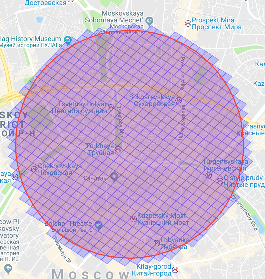
We can calculate a spherical segment (or “cap”) from the point of the center of the search and from the angle we just received. In fact, it is a circle on a sphere, but only three-dimensional.
Great, we have a “cap” inside which we need to look. But how? To do this, we will ask S2 to give us a list of storageLevel level cells that completely cover our circle or our “cap”.
It looks like this:
It remains only to walk through the received cells and get-s in the B-tree to get all the users that are inside.
For the test, we will create an index and several users. Three closer, two - away. And let us check that in the case of a small radius only three users return, and in the case of a larger radius, all. Hooray! Our simple little program works.
But there is one rather obvious drawback. In the case of a large search radius and low population density, it will be necessary for getters to check very, very many cells. It is not so fast.
Recall that we asked S2 to cover our “cap” with exactly the cells of the storageLevel level. But since these cells are rather small, they turn out a lot.
We can ask S2 to cover the “cap” with cells of different levels; then you get something like this:
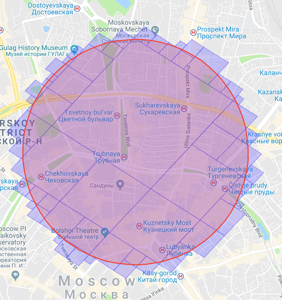
As you can see, S2 uses a larger cage inside the circle, and a smaller one at the edges. In sum, the cells become smaller.
But in order to find users from larger cells in our B-tree, we can no longer use Get. We need to ask S2 for each large cell the number of the first internal cell of our storageLevel level and the number of the last one and look for it using the range scan, that is, the query “from” and “to”.
The change is insignificant, but let's look at it in the process. We write simple benchmarks, which are engaged in the search cycle, and run them.
Our small change led to an acceleration of three orders of magnitude. Not bad!
We have considered the super-simple implementation of the search by radius. Let's now quickly go through the same simple implementation of geofencing, that is, determining which polygon we are in or which polygon is closest to us.
Here in our index, we will similarly need a B-tree, but in addition to it we will have a global map of all added polygons.
In the B-tree nodes, as before, we will store the list, but only now polygons that are in the storageLevel level cell.
In this example, we will have the functions of adding a polygon to an index, searching for a polygon in which we are located, and searching for the nearest polygon.
Let's start by adding a polygon. The polygon is given by the list of vertices, and S2 expects that the order of the vertices will be counterclockwise. But in case of an error, we will have a function of “normalization”, which, as it were, turns it inside out.
We will convert the list of vertex points into a Loop, and then into a polygon. The difference between them is that a polygon can consist of several loop-s, have a hole, for example, like a donut.
As in the previous example, we will ask S2 to cover our polygon with cells and add each of the returned cells to B-tree. Well, in the global map.
The search function of the polygon we are in is trivial in this example. As before, we transform the search coordinate in CellID at the storageLevel level and find or not find this cell in the B-tree.
Finding the nearest polygon is a bit more difficult. First, we will try to determine if suddenly we are already in some kind of testing ground. If not, then we will search by increasing radius (below I will show how it looks). Well, when we find the nearest polygons, we filter them and find the closest one, by calculating the distance to each of the found and taking the one that is the smallest.
What does “over increasing radius” mean? In the first picture you see the orange cell - the center of our search. First we will try to find the nearest polygon in all the adjacent cells (they are gray in the picture). If we don’t find anything there, we’ll move away to another level, as in the second picture. And so on.
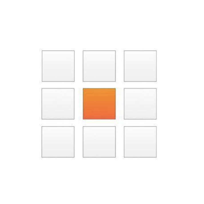
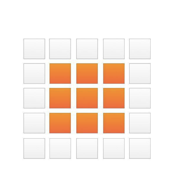
"Neighbors" gives us the function AllNeighbors. Unless you need to filter the cells and remove those that we have already viewed.
That's all. For this example, I also wrote a test, and it passes successfully.
If you are interested in looking at it or at full examples, you can find them here along with the slides.
If you ever need to write a search service that works with coordinates or some more complex geographic objects, and you don’t want or can’t use ready-made DBMS like PostGIS, think about S2.
This is a cool and simple tool that will give you basic things and a framework for working with coordinates and the globe. We in Badoo love S2 very much and recommend it in every possible way.
Thank!
Upd: And here comes the video!
My name is Marco, I work in Badoo on the Platform team. Not so long ago, on GopherCon Russia 2018, I told you how to work with coordinates. For those who do not like to watch the video (and of all those interested, of course), I publish a text version of my report.
')
Introduction
Now most people in the world have a smartphone with constant access to the Internet. Speaking in numbers, in 2018 almost 5 billion people will have a smartphone, and 60% of them use the mobile Internet.
These are huge numbers. It became easy and simple for companies to receive user coordinates. These ease and accessibility have spawned (and continue to spawn) a huge number of services based on coordinates.
We all know companies like Uber , games that have conquered the world, such as Ingress and Pokemon Go . But what is there, in any banking application, you can see ATMs or discounts nearby.
We at Badoo are also very active in using coordinates to provide our users with the best, relevant and interesting service for them. But what kind of use are we talking about? Let's look at examples of services that we have.
Badoo Geo Services
First example: Meetmaker and Geousers
Badoo is first of all dating. A place where people get to know each other. One of the important criteria when searching for people is the distance. Indeed, in most cases, a girl from Moscow wants to meet a boy who is a couple of kilometers away from her, or at least also lives in Moscow, and not in far Vladivostok.
Services that pick you people for a “yes / no game” or show users around are searching for people with the criteria that are appropriate for you within a certain radius of you.
Second example: Geoborder
In order to answer the questions in which city the user is located, in which country or, more precisely, for example, at which airport or at which university, we use the Geoborder service, which deals with the so-called geofencing .
The easiest way to answer these questions would be to consider the distance from the user to the city center or the center of the university, but this approach is very inaccurate and depends on a large number of boundary conditions.
Therefore, we have drawn very precise borders of countries, cities, important objects (for example, universities and airports, of which I spoke). These borders are defined by polygons. Having a set of such boundaries, we can understand whether the user is inside a polygon, or find the nearest polygon to it. Accordingly, we can tell in which city he is, or find the city nearest to him.
Third example: Bumpd
We have a very popular feature called Bumped Into, which in the background constantly searches for users to intersect in time and space and shows you that you regularly visit the same place at the same time with this boy or this girl walk regularly the same way. This feature is very popular with users, because it is another reason to get acquainted with the topic with which you can start a conversation.
Fourth example: Geocache - caching geo-information that is expensive to "get"
Well, the last example I’ll mention is related to caching geo-information. Imagine that you are using data from, for example, Booking.com, which provides you with information about hotels around, but to go to Booking.com every time is too long. Your internet pipe is probably quite narrow, like the pit of this gopher. Perhaps the service you go to for data takes money for each request and you want to save a little.
In this case, it would be nice to have a caching layer, which significantly reduces the number of requests to a slow or expensive service, and will provide a very similar API to the outside. A service that will understand that he already knows about all or most of the hotels in a given area, these data are relatively fresh, and, accordingly, you can not get behind them in an external service. Such tasks are solved in our service called Geocache.
Features of geo-services
We have already understood that there are a lot of coordinates, coordinates are important, and on the basis of them you can make a lot of interesting services. So what's next? What is actually the matter? How do the coordinates differ from any other information received from the user?
And I would say two features.
First, the geo-data is three-dimensional, or rather two-dimensional, because in the general case we are not interested in height. They consist of latitude and longitude, and the search most often goes simultaneously on both. Imagine searching in any area. Standard indexes in common DBMSs are not optimal for this use.
Secondly, many tasks require more complex data types such as polygons, which we discussed above using the example of the Geoborder service in Badoo. Polygons, of course, are composed of vertex coordinates, but require additional processing, and search queries for such data types are also more complicated. We have already seen the query "Find the nearest polygon to a point" or "Find a polygon that includes this point."
Why write your service
In order to comply with these features, many DBMSs include special indexes, sharpened for multidimensional data, and additional functions that allow you to work with objects such as polygons or broken lines.
Probably the most striking example is PostGIS - an extension to the popular PostgreSQL DBMS, which has the most extensive capabilities for working with coordinates and geography.
But using a ready-made DBMS is not the only and not always the best solution.
If you do not want to divide the business logic of your service between it and the DBMS, if you want something that is not available in the DBMS, if you want to fully manage your service and not be limited to scaling any DBMS, for example, then you can want to embed the ability to search and work with geo-data in your service.
Such an approach is undoubtedly more flexible, but it can be much more complicated, because the DBMS is an all-in-one solution, and many infrastructure-type replications are already done for you. Replications and, in fact, algorithms and indices for working with coordinates.
But not so scary. I would like to introduce you to the library, which implements most of what you need. Which is a kind of cube, easily embedded wherever you need to work with the geometry on the sphere or search by coordinates. With a library called S2 .
S2
S2 is a library for working with geometry (including on a sphere), which provides very convenient possibilities for creating geo-indices.
Until recently, S2 was virtually unknown and had very poor documentation, but not so long ago, Google decided to " re-release " it in open-source, adding to the layout with a promise to support and develop the product.
The main version of the library is written in C ++ and has several official ports or versions in other languages, including the Go version. The go-version today is not 100% realizing everything that is in the C ++ version, but what is there is enough to implement most things.
In addition to Google, the library is actively used in companies such as Foursquare , Uber , Yelp , and of course Badoo . And among the products that use the library inside, you can highlight the well-known MongoDB.
But so far I have not said anything sensible about why S2 is convenient and why it makes it easy to write services with a geo search. Let me fix and immerse myself a bit in the guts before we look at two examples.
Projection
Usually geography involves the use of one of the most common projections of the globe on a plane. For example, we all know the projection of the Mercator . The disadvantage of this approach is that any projection somehow has distortions. Our globe with you is not very much like a plane.
Recall the famous picture with a comparison of Russia and Africa. On the maps, Russia is huge, and in fact, the area of Africa is already twice the area of Russia! This is just an example of the distortion of the Mercator projection.
S2 solves this problem by using exclusively spherical projection and spherical geometry. Of course, the Earth is also not quite a sphere, but distortions in the case of a sphere can be neglected for most tasks.
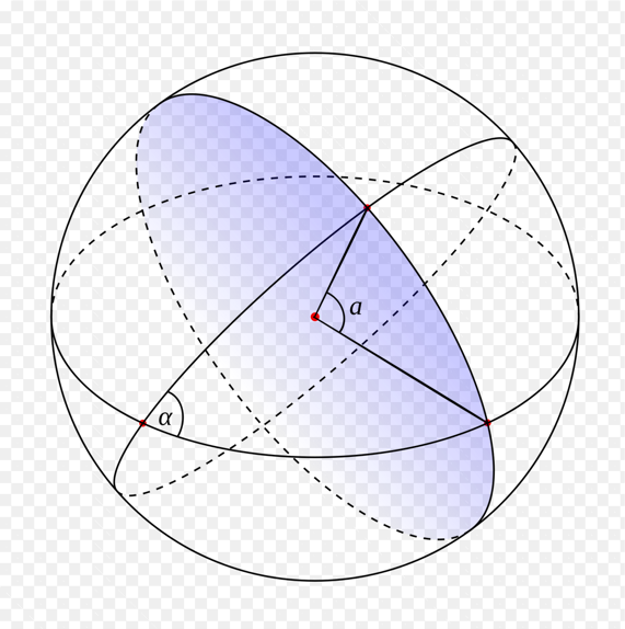
We will work with a unit, or unit-sphere , that is, with a sphere of radius 1 and we will use such concepts as the central angle , the spherical rectangle and the spherical segment .
The name S2 is derived from the mathematical notation denoting the unit sphere.
But you should not be afraid, as the library takes on almost all the mathematics.
Hierarchical cells (cells)
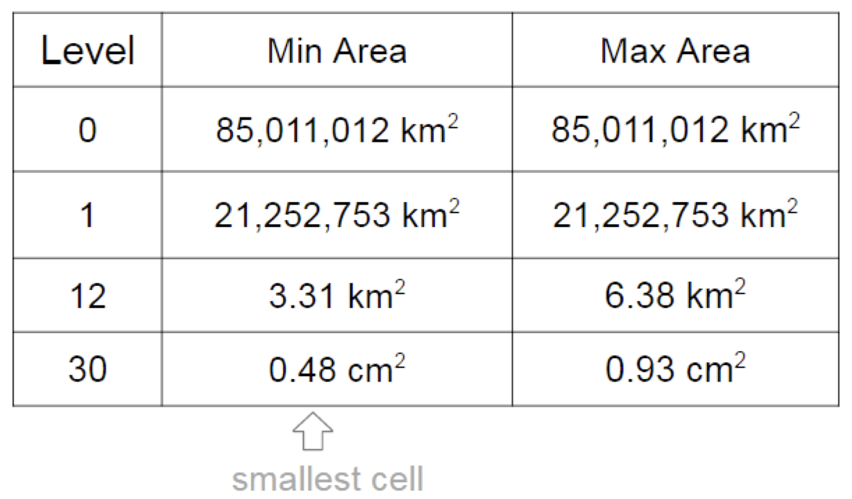
The second (and most important) feature of the library is the concept of hierarchical partitioning of the globe into cells (in English - cells).
The division is hierarchical, that is, there is such a thing as a level (or level) of a cell. And at one level, the cells are about the same size.
Cells can set any point on Earth. If you use a cell of the maximum, 30th level, which is smaller than a centimeter in width, then the accuracy, as you understand, will be very high. The lower level cells can set the same point, but the accuracy will be less. For example, 5 m by 5 m.
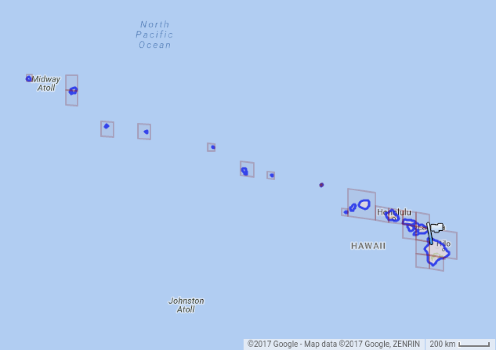
Cells can be set not only points, but also more complex objects such as polygons and some areas (in the picture you, for example, see Hawaii). In this case, such figures will be given by sets of cells (possibly at different levels).
Such a partition is very compact: each cell can be encoded with one 64-bit number.
Hubert Curve
I mentioned that the cell is defined by one 64-bit number. Here it is! It turns out that a coordinate or a point on Earth, which by default is given by two coordinates, with which we are inconvenient to work with standard methods, can be given with a single number. But how to achieve this? Let's get a look…
How does the hierarchical division of the sphere occur?
We first surround the sphere with a cube and project it onto all six of its faces, slightly modifying the projection on the move to remove distortion. This is level 0. Then we can divide each of the six faces of the cube into four equal parts - this is level 1. And each of the four parts that we can get can be further divided into four equal parts - level 2. And so on until level 30.
But at this stage, we still have two-dimensionality. And here we come to the aid of a mathematical idea from the distant past. At the end of the 19th century, David Hilbert came up with a way to fill any space with a one-dimensional line that turns, collapses and thus fills the space. The Hilbert curve is recursive, which means that precision or density can be chosen. Any small piece we can fill up more tightly if necessary.
We can fill our two-dimensional space with such a curve. And if we now take this curve and stretch it into a straight line (as if we are pulling a thread), we will get a one-dimensional object describing a multi-dimensional object, a one-dimensional object or a coordinate on this line, which is convenient and easy to work with.
Something like the filling of the Hilbert curve of the Earth at one of the middle levels:
Another feature of the Hilbert curve is the fact that the points that are near on the curve are near and in space. The reverse is not always the case, but mostly true. And we will actively apply this feature too.
Encoding to 64-bit variable
But why can we encode any cell with a single 64-bit number, which, by the way, is called CellID? Let's get a look.
We have six faces of the cube. Six different values can be encoded in three bits. Recall logarithms .
Then we divide each of the six faces into four equal parts 30 times. To set one of the four parts into which we divide the cell at each level, two bits are enough for us.
Total 3 + 2 * 30 = 63. And we will set one extra bit at the end in order to know and quickly understand what level a cell is assigned to this CellID.
What do all these partitions and coding of the Hilbert curve into one number give us?
- We can encode any point on the globe with one CellID. Depending on the level, we get different accuracy.
- We can encode any two-dimensional object on the globe with one or several CellID. Similarly, we can play with precision by varying the levels.
- The property of the Hilbert curve, which consists in the fact that the points that are near on it are near and in space, and the fact that we have a CellID is just a number, allows us to use an ordinary B-tree for searching. Depending on what we are looking for (point or area), we will use either get, or range scan, that is, the search “from” and “to”.
- Splitting the globe into levels gives us a simple sharding framework for our system. For example, at the zero level we can divide our service into six instances, at the first level - into 24, etc.
Now, to consolidate this theoretical knowledge, let's look at two examples. We will write two simple services, and the first one is just a search for “around”.
Examples
Let's write a search service for people around
We will make a search index. We need a function to create an index, a function to add a person to the index and, in fact, a search function. Well, the test.
type Index struct {} func NewIndex(storageLevel int) *Index {} func (i *Index) AddUser(userID uint32, lon, lat float64) error {} func (i *Index) Search(lon, lat float64, radius uint32) ([]uint32, error) {} func TestSearch(t *testing.T) {} The user is defined by his ID and coordinates, and the search - by the coordinates of the search center and the search radius.
In the index, we need a B-tree, in the nodes of which we will store a cell of the storageLevel level and a list of users in this cell. The storageLevel cell level is the choice between initial search accuracy and performance. In this example, we will use a cell of about 1 km in size per 1 km. The Less function is necessary for B-tree to work, so that the tree can understand which of our values is smaller and which of them is greater.
type Index struct { storageLevel int bt *btree.BTree } type userList struct { cellID s2.CellID list []uint32 } func (ul userList) Less(than btree.Item) bool { return uint64(ul.cellID) < uint64(than.(userList).cellID) } Now let's look at the add user function.
func (i *Index) AddUser(userID uint32, lon, lat float64) error { latlng := s2.LatLngFromDegrees(lat, lon) cellID := s2.CellIDFromLatLng(latlng) cellIDOnStorageLevel := cellID.Parent(i.storageLevel) // ... } Here we see S2 in action for the first time. We convert our coordinates, given in degrees, to radians, and then to CellID, which corresponds to these coordinates at the maximum level of 30th (that is, with the minimum cell size), and convert the resulting CellID to CellID of the level at which we will keep people. If you look "inside" of this function, we will see just zeroing of several bits. Remember how CellID is encoded.
func (i *Index) AddUser(userID uint32, lon, lat float64) error { // ... ul := userList{cellID: cellIDOnStorageLevel, list: nil} item := i.bt.Get(ul) if item != nil { ul = item.(userList) } ul.list = append(ul.list, userID) i.bt.ReplaceOrInsert(ul) return nil } Then we just need to add this user to the appropriate cell in the B-tree. Either first, or at the end of the list, if someone is already there. Our simple index is ready.
Go to the search function. The first transformations are similar, but instead of a cell, we obtain the “dot” object by coordinates. This is the center of our search.
func (i *Index) Search(lon, lat float64, radius uint32) ([]uint32, error) { latlng := s2.LatLngFromDegrees(lat, lon) centerPoint := s2.PointFromLatLng(latlng) centerAngle := float64(radius) / EarthRadiusM cap := s2.CapFromCenterAngle(centerPoint, s1.Angle(centerAngle)) // ... return result, nil } Further along the radius given in meters, we get the central angle. This is the angle from the center of the sphere. The transformation in this case is simple: it is enough to divide our radius in meters by the radius of the Earth in meters.
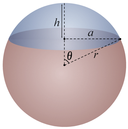
We can calculate a spherical segment (or “cap”) from the point of the center of the search and from the angle we just received. In fact, it is a circle on a sphere, but only three-dimensional.
Great, we have a “cap” inside which we need to look. But how? To do this, we will ask S2 to give us a list of storageLevel level cells that completely cover our circle or our “cap”.
func (i *Index) Search(lon, lat float64, radius uint32) ([]uint32, error) { // ... rc := s2.RegionCoverer{MaxLevel: i.storageLevel, MinLevel: i.storageLevel} cu := rc.Covering(cap) // ... return result, nil } It looks like this:
It remains only to walk through the received cells and get-s in the B-tree to get all the users that are inside.
func (i *Index) Search(lon, lat float64, radius uint32) ([]uint32, error) { // ... var result []uint32 for _, cellID := range cu { item := i.bt.Get(userList{cellID: cellID}) if item != nil { result = append(result, item.(userList).list...) } } return result, nil } For the test, we will create an index and several users. Three closer, two - away. And let us check that in the case of a small radius only three users return, and in the case of a larger radius, all. Hooray! Our simple little program works.
func prepare() *Index { i := NewIndex(13 /* ~ 1km */) i.AddUser(1, 14.1313, 14.1313) i.AddUser(2, 14.1314, 14.1314) i.AddUser(3, 14.1311, 14.1311) i.AddUser(10, 14.2313, 14.2313) i.AddUser(11, 14.0313, 14.0313) return i } func TestSearch(t *testing.T) { indx := prepare() found, _ := indx.Search(14.1313, 14.1313, 2000) if len(found) != 3 { t.Fatal("error while searching with radius 2000") } found, _ = indx.Search(14.1313, 14.1313, 20000) if len(found) != 5 { t.Fatal("error while searching with radius 20000") } } $ go test -run 'TestSearch$' PASS ok github.com/mkevac/gophercon-russia-2018/geosearch 0.008s But there is one rather obvious drawback. In the case of a large search radius and low population density, it will be necessary for getters to check very, very many cells. It is not so fast.
Recall that we asked S2 to cover our “cap” with exactly the cells of the storageLevel level. But since these cells are rather small, they turn out a lot.
We can ask S2 to cover the “cap” with cells of different levels; then you get something like this:
rc := s2.RegionCoverer{MaxLevel: i.storageLevel} cu := rc.Covering(cap) As you can see, S2 uses a larger cage inside the circle, and a smaller one at the edges. In sum, the cells become smaller.
But in order to find users from larger cells in our B-tree, we can no longer use Get. We need to ask S2 for each large cell the number of the first internal cell of our storageLevel level and the number of the last one and look for it using the range scan, that is, the query “from” and “to”.
func (i *Index) SearchFaster(lon, lat float64, radius uint32) ([]uint32, error) { // ... for _, cellID := range cu { if cellID.Level() < i.storageLevel begin := cellID.ChildBeginAtLevel(i.storageLevel) end := cellID.ChildEndAtLevel(i.storageLevel) i.bt.AscendRange(userList{cellID: begin}, userList{cellID: end.Next()},func(item btree.Item) bool { result = append(result, item.(userList).list...) return true }) } else { // ... } } return result, nil } The change is insignificant, but let's look at it in the process. We write simple benchmarks, which are engaged in the search cycle, and run them.
var res []uint32 func BenchmarkSearch(b *testing.B) { indx := prepare() for i := 0; i < bN; i++ { res, _ = indx.Search(14.1313, 14.1313, 50000) } } func BenchmarkSearchFaster(b *testing.B) { indx := prepare() for i := 0; i < bN; i++ { res, _ = indx.SearchFaster(14.1313, 14.1313, 50000) } } Our small change led to an acceleration of three orders of magnitude. Not bad!
$ go test -bench=. goos: darwin goarch: amd64 pkg: github.com/mkevac/gophercon-russia-2018/geosearch BenchmarkSearch-8 500 3097564 ns/op BenchmarkSearchFaster-8 200000 7198 ns/op PASS ok github.com/mkevac/gophercon-russia-2018/geosearch 3.393s Let's write a geofencing service
We have considered the super-simple implementation of the search by radius. Let's now quickly go through the same simple implementation of geofencing, that is, determining which polygon we are in or which polygon is closest to us.
Here in our index, we will similarly need a B-tree, but in addition to it we will have a global map of all added polygons.
type Index struct { storageLevel int bt *btree.BTree polygons map[uint32]*s2.Polygon } func NewIndex(storageLevel int) *Index { return &Index{ storageLevel: storageLevel, bt: btree.New(35), polygons: make(map[uint32]*s2.Polygon), } } In the B-tree nodes, as before, we will store the list, but only now polygons that are in the storageLevel level cell.
type IndexItem struct { cellID s2.CellID polygonsInCell []uint32 } func (ii IndexItem) Less(than btree.Item) bool { return uint64(ii.cellID) < uint64(than.(IndexItem).cellID) } In this example, we will have the functions of adding a polygon to an index, searching for a polygon in which we are located, and searching for the nearest polygon.
func (i *Index) AddPolygon(polygonID uint32, vertices []s2.LatLng) error {} func (i *Index) Search(lon, lat float64) ([]uint32, error) {} func (i *Index) SearchNearest(lon, lat float64) ([]uint32, error) {} Let's start by adding a polygon. The polygon is given by the list of vertices, and S2 expects that the order of the vertices will be counterclockwise. But in case of an error, we will have a function of “normalization”, which, as it were, turns it inside out.
func (i *Index) AddPolygon(polygonID uint32, vertices []s2.LatLng) error { points := func() (res []s2.Point) { for _, vertex := range vertices { point := s2.PointFromLatLng(vertex) res = append(res, point) } return }() loop := s2.LoopFromPoints(points) loop.Normalize() polygon := s2.PolygonFromLoops([]*s2.Loop{loop}) // ... return nil } We will convert the list of vertex points into a Loop, and then into a polygon. The difference between them is that a polygon can consist of several loop-s, have a hole, for example, like a donut.
As in the previous example, we will ask S2 to cover our polygon with cells and add each of the returned cells to B-tree. Well, in the global map.
func (i *Index) AddPolygon(polygonID uint32, vertices []s2.LatLng) error { // ... coverer := s2.RegionCoverer{MinLevel: i.storageLevel, MaxLevel: i.storageLevel} cells := coverer.Covering(polygon) for _, cell := range cells { // ... ii.polygonsInCell = append(ii.polygonsInCell, polygonID) i.bt.ReplaceOrInsert(ii) } i.polygons[polygonID] = polygon return nil } The search function of the polygon we are in is trivial in this example. As before, we transform the search coordinate in CellID at the storageLevel level and find or not find this cell in the B-tree.
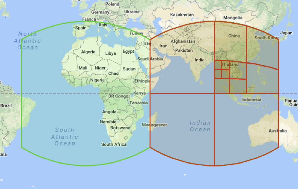
func (i *Index) Search(lon, lat float64) ([]uint32, error) { latlng := s2.LatLngFromDegrees(lat, lon) cellID := s2.CellIDFromLatLng(latlng) cellIDOnStorageLevel := cellID.Parent(i.storageLevel) item := i.bt.Get(IndexItem{cellID: cellIDOnStorageLevel}) if item != nil { return item.(IndexItem).polygonsInCell, nil } return []uint32{}, nil } Finding the nearest polygon is a bit more difficult. First, we will try to determine if suddenly we are already in some kind of testing ground. If not, then we will search by increasing radius (below I will show how it looks). Well, when we find the nearest polygons, we filter them and find the closest one, by calculating the distance to each of the found and taking the one that is the smallest.
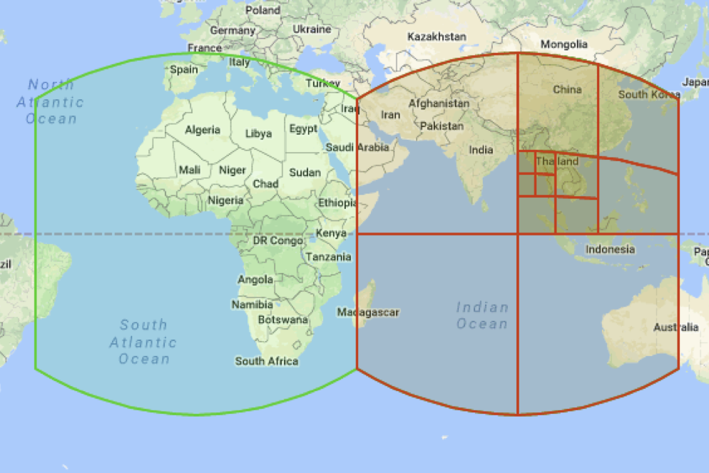
func (i *Index) SearchNearest(lon, lat float64) ([]uint32, error) { // ... alreadyVisited := []s2.CellID{cellID} var found []IndexItem searched := []s2.CellID{cellID} for { found, searched = i.searchNextLevel(searched, &alreadyVisited) if len(searched) == 0 { break } if len(found) > 0 { return i.filter(lon, lat, found), nil } } return []uint32{}, nil } What does “over increasing radius” mean? In the first picture you see the orange cell - the center of our search. First we will try to find the nearest polygon in all the adjacent cells (they are gray in the picture). If we don’t find anything there, we’ll move away to another level, as in the second picture. And so on.
"Neighbors" gives us the function AllNeighbors. Unless you need to filter the cells and remove those that we have already viewed.
func (i *Index) searchNextLevel(radiusEdges []s2.CellID, alreadyVisited *[]s2.CellID) (found []IndexItem, searched []s2.CellID) { for _, radiusEdge := range radiusEdges { neighbors := radiusEdge.AllNeighbors(i.storageLevel) for _, neighbor := range neighbors { if in(*alreadyVisited, neighbor) { continue } *alreadyVisited = append(*alreadyVisited, neighbor) searched = append(searched, neighbor) item := i.bt.Get(IndexItem{cellID: neighbor}) if item != nil { found = append(found, item.(IndexItem)) } } } return } That's all. For this example, I also wrote a test, and it passes successfully.
If you are interested in looking at it or at full examples, you can find them here along with the slides.
Conclusion
If you ever need to write a search service that works with coordinates or some more complex geographic objects, and you don’t want or can’t use ready-made DBMS like PostGIS, think about S2.
This is a cool and simple tool that will give you basic things and a framework for working with coordinates and the globe. We in Badoo love S2 very much and recommend it in every possible way.
Thank!
Upd: And here comes the video!
Source: https://habr.com/ru/post/352754/
All Articles