Procedural worlds from simple tiles

In this post I will describe two algorithms for creating complex procedural worlds from simple sets of colored tiles and based on the constraints of the location of these tiles. I will show how, with a neat design of these tile sets, you can create interesting procedurally generated content, for example, landscapes with cities or dungeons with a complex internal structure. The video below shows a system that creates a procedural world based on the rules encoded in 43 color tiles.


The image below shows a set of tiles (tileset), on the basis of which the world is generated from the video. The world is equipped with notes that will help to present it in a real environment.


We can define tiling as the final grid, in which each of the tiles is in its own grid cell. We define the correct world as a world in which the colors along the edges of neighboring tiles must be the same.


The tiling has only one iron rule: the colors of the edges of the tiles must match. The entire high-level structure evolves based on this rule.
')
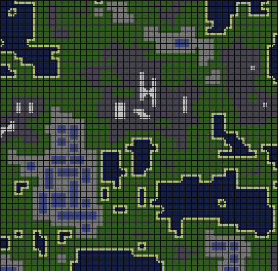
The correct tiling looks like this:


This is a tiling, which should represent a map with water, coasts, grass, cities with buildings (blue rectangles), and mountains with snowy peaks. Black lines show borders between tiles.

I think this is an interesting way of describing and creating worlds, because very often the top-down approach is used in procedural generation algorithms. For example, in L-systems, a recursive description of an object is used, in which high-level, large parts are determined earlier than low-level ones. There is nothing wrong with this approach, but I think it is interesting to create sets of tiles that can encode only simple low-level relationships (for example, sea water and grass should be separated by the coast, buildings should have only convex corners at 90 degrees) and watch the emergence of high-level patterns (for example, square buildings).

Tiling is an NP-complete task of satisfying constraints

For a reader familiar with the problems of satisfying constraints (CSP), it is already obvious that the tiling of a finite world is an OWL. In PWD, we have a set of variables, a set of values ​​that each variable can take (called its definition domain), and a set of constraints. In our case, the variables are the coordinates on the map, the definition of each variable is tileset, and the limitations are that the edges of the tiles must correspond to the edges of the neighbors.

It is intuitively clear that the task of creating a non-trivial tiling correctly is difficult, since tilesets can encode arbitrary extensive dependencies. When we consider a tileset as a whole, from a formal point of view, this is an NP-complete task of satisfying constraints. The naive algorithm for creating tilings consists of an exhaustive search for the space of tilings and is executed in exponential time. There is a hope that we can create interesting worlds on the basis of tilesets solved by a search that can be accelerated by heuristics. Another option is to create tilings that are approximately correct, but contain a small number of incorrect locations. I found two algorithms that work well with some interesting tilesets, and I’ll describe them below.

Method 1: greedy arrangement with reverse transitions

Select random places and put the appropriate tiles there. If we get stuck, remove some of them and try again.





t <-
l <- t,
l




The first attempt to create a tiling from a tileset was that the entire grid was in an unresolved state, after which I iteratively placed a random tile in a suitable place for it, or, if there were no suitable places, assigned a small area next to the unsolved tile and continued the greedy arrangement of the tiles. “Greedy arrangement” is a strategy of tile arrangement as long as its faces correspond to the tiles already placed, regardless of whether such an arrangement will create partial tiling that cannot be completed without replacing the already set tiles. When such a situation arises and we can no longer arrange tiles, we must delete some of the previously located tiles. But we do not know which of them is best to remove, because if we could solve the problem, then, probably, we could also solve the problem of the correct arrangement of tiles in the first place. To give the algorithm one more chance to find a suitable tile for a given area, we assign the state “unsolved” to all the tiles around the unresolved point and continue to carry out the strategy of the greedy arrangement. We hope that sooner or later the correct tiling will be found, but there is no guarantee of this. The algorithm will be executed until the correct tiling is found, which can take infinite time. He does not have the ability to determine that tileset is undecidable.

There are no guarantees that the algorithm will complete its work. A simple tileset with two tiles that have no common colors will cause the algorithm to perform an infinite loop. An even simpler case would be one tile with different colors above and below. It will be reasonable to find some way to determine that tile sets cannot create the correct tilings. We can say that a tileset is definitely true if it can pave an infinite plane. In some cases, it can be easily proved that a tileset can or cannot pave an infinite plane, but in the general case this problem is unsolvable. Therefore, the task of the designer is to create a tileset that can create the correct tiling.

This algorithm is unable to find good solutions for the dungeon tileset from the video at the beginning of the post. It works well with simpler tilesets. We would like to learn how to solve more complex tilesets with a variety of possible types of transitions between tiles and various coded rules (for example, that roads must begin and end next to buildings).

We need an algorithm that can look ahead and create tile locations, somehow aware of the ways in which these locations are open for future tile locations. This will allow us to effectively solve difficult tilesets.

In terms of satisfying the constraints

This algorithm is similar to search with a reverse transition. At each step, we try to assign one variable. If we cannot, then we cancel the assignment of a variable and all variables that are attached to it by constraints. This is called “backjumping” and is different from backtracking, in which we cancel the assignment of one variable at a time until we can continue to make the correct assignments. When you go back, we generally cancel the assignment of variables in the reverse order of their assignment, however, when going back, we cancel the assignment of variables according to the structure of the task in question. It is logical that if we cannot place any tile at a specific point, then we must change the location of neighboring tiles, since their location created an unsolvable situation. Returning back instead can lead us to cancel the assignment of variables that are spatially far apart, but have been assigned recently.

This search does not use any methods of local integrity. That is, we do not attempt to locate the tiles, which will later lead to an unsolvable situation, even through a single search step in the future. It is possible to accelerate the search by tracking the influence that the location will have on the possible locations in several tiles from the current point. At the same time, it is hoped that this will allow the search not to spend so much time on the cancellation of its work. This is exactly what our algorithm does.

Method 2: location with the greatest restrictions and distribution of local information

We preserve the probability distribution for tiles at each point, introducing non-local changes to these distributions when deciding on the location. Never backtracking.


Next, I will describe an algorithm that is guaranteed to be completed and creates more visually pleasing results for all the tiles I have tested. In addition, it can create almost true tilings for much more complex tilesets. The compromise here is that this algorithm does not guarantee that the output will always be correct tiling. The Optimizations section describes optimizations that allow you to perform this algorithm more quickly, even with larger tilesets and maps.

The complexity of creating the right tiling strongly depends on the number of transitions necessary for the transition between two types of tiles. In a simple tileset there can only be sand, water and grass. If grass and water cannot touch each other, then there must be a transition to the sand between them. This is a simple example that the algorithm presented earlier can easily solve. In a more complicated case, multiple built-in levels of tile types can be represented. For example, we may have deep water, water, sand, grass, a high plain, a mountain, and a snowy peak. In order for all these types of tiles to appear on the map, it is necessary to have seven transitions, if we assume that these types cannot touch each other except in the order I specified. Additional complexity can be added by creating tiles that naturally create extensive dependencies between tiles, for example, roads that must start and end next to certain types of tiles.

Intuitively, the algorithm for this task should be able to “look ahead” and consider at least a few transitions that may be the consequences of the chosen location. To do this, you can think of a tile map as a probability distribution for tiles at each point. When the algorithm places a tile, it updates the probability distribution around this tile in response to its location in such a way that it increases the likelihood of neighboring tiles, which can probably be compatible with the current location.

For example, if there is a water tile on the card, then the tiles next to it must contain water. Tiles near them can also contain water, but there are other probabilities, for example, grass, if the coast is placed near the original water tile. The further we move away from the tile located, the more types of tiles it becomes possible. To take advantage of this observation, we can count the number of ways in which we can reach the location of each tile next to the source tile. In some cases, only a single sequence of transitions can lead to the transition of one tile to another at a given distance. In other cases, there may be many different sequences of transitions. After the location of the tile, we can determine the probability distribution of tiles in neighboring points, counting the number of ways we can make the transition from the tile, which we have arranged, to neighboring tiles. The “look ahead” performed by this algorithm is tracking of such numbers of transitions and their processing as probability distributions from which one can choose available new tiles.


At each step, the algorithm examines all the unresolved tile locations, each of which has a probability distribution over the tiles, and selects one place to “converge” to the tile. He chooses a distribution from a map with minimal entropy. In the case of multinomial distributions with low entropy, the probabilities are usually concentrated in several modes, therefore the convergence of these first ones leads to the effect of placing tiles, for which some of the limitations already exist. That is why the algorithm places the tiles next to the tiles that we decided first.

This is the most efficient algorithm that I managed to implement for this task. It has another advantage: it creates beautiful visualizations while performing. Perhaps there is a way to improve this algorithm by entering some form of reversion. If there is an incorrect point in the resulting finished tiling, then canceling the locations of neighboring tiles and resampling from the resulting distributions at their points may allow finding a fix for this ready tiling. Of course, if you want to continue searching until you find the correct tiling, then exceed the limits of the specified guaranteed execution time.

Optimization

The most important operation of this method is to update the probabilities around the tile located. One approach would be to count the possible transitions "out" from the tile located each time the tile is located. This will be very slow, since for each point of the map, to which the new probabilities will extend, it will be necessary to consider many pairs of transitions. Obvious optimization will not be spreading to the entire map. A more interesting optimization is the caching of influence that each tile arrangement will have on points around it, so that each tile arrangement simply performs a search to check what types of changes the arrangement makes to adjacent probabilities, followed by applying this change with some simple operations. Below I will describe my implementation of this optimization method.

Imagine a tile placed on a completely empty card. This location will update the adjacent tile probabilities. We can consider these updated distributions as having the previous distribution defined by the previous tile locations. If several tiles are placed, this previous distribution will be shared. I approximate this posterior probability taking into account the previous joint as the product of distributions for each location in the past.


To realize this, I will imagine that when the tile is located on an empty map, it introduces significant changes in the distribution of neighboring points of the map. I will call these updates the sphere of a tile, that is, the sphere of influence of a tile projected around it when it is placed on an empty map. When two tiles are located next to each other, their spheres interact and create finite distributions, which are influenced by both locations. Given that many tiles can be located near a given unresolved place, there will be a large number of interacting constraints, making a counting decision to determine the probability of different tiles appearing at this point as a very slow process. What if, instead, we consider only a simple model of interaction between previously calculated tile spheres that were already located on the map?


With the location of the tile, I update the probability map for each element, multiplying the distribution of the sphere of this tile by each point of the map by the distribution already stored at that point of the map. It may be helpful to look at an example of what this can do with the distribution map. Suppose a given map point currently has a distribution that can equally select grass or water, and we place a water tile next to this point. The sphere of the water tile will have a high probability of water near the water tile and a low probability of grass tile. When we multiply these distributions element by element, the likelihood of water will be high as a result, because it is the product of two large probabilities, but the likelihood of grass will be low, because it is the product of a high probability stored on the map, with a low probability stored in the field.


This strategy allows us to efficiently approximate the effect that each tile arrangement should have on a probability map.

In terms of satisfying the restrictions

In order to effectively solve problems of satisfying constraints, it is often reasonable to track those assignments of other variables that become impossible when assigning a particular variable. This principle is called the introduction of local compatibility conditions. Introducing some kind of local compatibility avoids assigning a variable a value when assigning an adjacent variable an incompatible value when it is necessary to go back. Such transformations are related to the field of methods of propagation of restrictions in the literature on CBD. In our algorithm, we spread information to a small area of ​​the map each time we place a tile. The information disseminated informs which tiles can and cannot appear next to each other. For example, if we have a mountain tile, then we know that there cannot be an open sea tile in two tiles of it, that is, the probability of a sea tile at all points of the map in two tiles from a tile located is zero. This information is recorded in the areas of which we spoke above. The spheres encode the local compatibility we want to impose.

By reducing the number of possible assignments of neighboring tiles, we significantly reduce the search space that the algorithm should process after each location. We know that in this small neighborhood all the probabilities of the appearance of tiles that are incompatible with the location are zero. This is analogous to removing these values ​​from the variable definition areas at these points. That is, each pair of neighboring points in the area around a tile has in its domain a certain tile that is compatible with some tile that is still in the domain of definition of neighbors. When two variables are connected by a constraint to the task of the PP, and their domains of definition contain only values ​​satisfying the constraint, they are said to have arc compatibility, that is, this method is actually an effective strategy for introducing arc compatibility.

In PWD, the “most limited” variable in a given partial assignment is the one with the least possible values ​​in the definition area. The principle of the location of a tile at a point by the minimum distribution of entropy on the map is similar to assigning the value to the most limited variable in the OIL, which is the standard heuristic of the ordering of variables when solving OAT using a search.

Tiller manipulation of changing tile selection probabilities

So far I have only talked about how to create the right tilings, but besides correctness, other properties may be required from the tiling. For example, we may need a certain ratio of the number of one type of tiles to another, or we want to ensure that not all tiles have the same type, even if such a tiling is correct. To solve this problem, both algorithms described by me receive as input the basic probability associated with each tile. The higher this probability, the more likely this tile will be present in the finished tiling. Both algorithms make a random selection from a collection of tiles, and I will simply add weights to this random selection according to the basic probabilities of the tiles.

Below is an example of using this principle. By changing the likelihood of a solid water tile, I can adjust the size and frequency of water appearing on the map.

Create your own tilesets

In short:

• clone my repository on github
• install Processing
• in the data / repository folder, change tiles.png
• use processing to open wangTiles.pde and click on the play button

With the help of the code laid out on github (you can change it, but do it at your own peril and risk - I wrote most of it in high school) you can create your own tilesets using the image editor and watch the tiling solver create worlds with them . Simply clone the repository and edit the image of dungeon.png, and then use Processing to launch wangTiles.pde and view the animation of the generated map. Below I will describe the “language” that this tiling solver needs.

Tilesets specification

Tiles are arranged in a grid of 4x4 cells. Each cell in the upper left 3x3 area contains a color tile, and the remaining 7 pixels contain tile metadata. Pixel under the center of the tile can be painted in red to comment out the tile and exclude it from the tileset. Solvers will never put it on the map. The upper pixel on the right side of the tile can be painted black to add all four tile turns to the tileset. , - , . , . . , .

, , , , .

«Most Constrained Placement with Fuzzy Arc Consistency» Wave Function Collapse Twitter @ExUtumno. This algorithm stores a map of “partially observable” assignments and, to create a final image, takes samples from them, which is similar to the distributions I keep for tiles. These approaches differ in some aspects. For each point of the map, this algorithm preserves binary potentials, and not multinomial distributions. In addition, it does not use cached "spheres" of the number of transitions needed to speed up the calculations, which I talked about in the "Optimization" section.

Conclusions and thanks

, , « » , - , , . . . , . , . , .

. . , .