Heading "We read articles for you." February - March 2018

Hi, Habr! We continue to publish reviews of research papers from members of the Open Data Science community from #article_essense. Want to get them before everyone else - join the community !

Articles for today:

1. Learning Semantic Segmentation with Diverse Supervision (University of Manitoba, Shanghai University, 2018)
2. TVAE: Triplet-Based Variational Autoencoder using Metric Learning (Stanford University, 2018)
3. Neural-Symbolic Learning and Reasoning: A Survey and Interpretation
4. Overcoming catastrophic forgetting in neural networks (DeepMind, Imperial College London, 2016)
5. Deep Image Harmonization (University of California, Adobe, 2017)
6. Accelerated Gradient Boosting (Sorbonne Université, Univ Rennes, 2018)

1. Learning Semantic Segmentation with Diverse Supervision

Authors: Linwei Ye, Zhi Liu, Yang Wang (University of Manitoba, Shanghai University, 2018)
→ Original article
Review author: Egor Panfilov (in Slak egor.panfilov)

In this article, the authors propose an architecture for learning CNN in the problem of semantic segmentation, which allows using data with different types of markup (pixel-by-pixel masks, bounding boxes, labels for the entire image) for training.

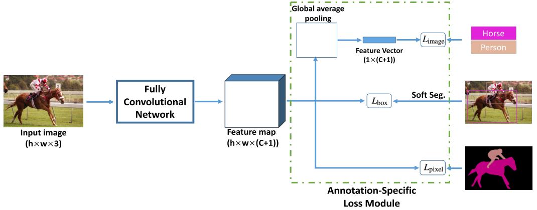
The architecture is an FCN receiving the tensor (h w 3) at the input, and the outstanding tensor (h w (C + 1)), i.e. with the same spatial dimensions as the original image. The output feature map is then used in three heads to calculate the loss: (1) L_image (global average pooling -> multi-category BCE loss), (2) L_bbox, (3) L_pixel (average pixel-by-pixel BCE).

L_bbox is one of the most interesting parts of the article. The problem here is how to turn a bbox for an object into a scalar-loss. The authors' approach is to generate an approximate object mask on the basis of bbox (tried by Grabcut, MCG, simple bbox fill, and UCM (ultrametric contour map)). UCM earned the best, or rather its version, where overlapping several bboxes a pixel is taken into account for each class (soft.segm.). The option where it is assigned to one class (hard.segm.) Proved to be a little worse. Mask generation by UCM works like this: (a) select contours according to UCM, (b) normalize by intensity, (c) set 3 treshhold values ​​(1/4, 2/4, 3/4), (d) start to fill concentric contours until we leave the area for some amount%. We assign label uncertain to the remnants of private masks for these treshholds - we ignore them when calculating the loss. Having the prediction of the network and the created reference mask, we consider the loss.

Experiments: the authors trained FCN and DeepLab at PASCAL VOC 2012, using various types of markup and in different proportions (masks: bbox: labels - from 1: 1: 1 to 1: 5: 10). The results show that bboxes do decently, but with very acidic markup (when there are very few pixel-pixel masks), the image-level labels also help.

2. TVAE: Triplet-Based Variational Autoencoder using Metric Learning

Authors: Haque Ishfaq, Assaf Hoogi, Daniel Rubin (Stanford University, 2018)
→ Original article
Review author: Egor Panfilov (in Slak egor.panfilov)

In the article, fresh blood from Stanford tries to make a contribution to the Deep Metric Learning area. Without answering the question why, and what problem they are trying to solve, the authors propose to take the VAE for the pictures, pull out the vector of meanings from the bottleneck (not paying attention to the dispersion), and add a triplet of loss over it. Thus, the network is trained on mixed losse: L_tv_ae = L_reconstruction + L_KL + L_triplet.

They teach MNIST with embedding dimensions 20 incomprehensible network with unclear what parameters an incomprehensible amount of time. Estimate the devil also knows how - by calculating after training the percentage of triplets on which the triplet loss is zero. The indicator for this "quality metric" is improving, which, generally speaking, is expected, since its reverse version was added to the loss function and, accordingly, tried to be minimized. As a final note, t-SNE embeddings on two approaches (VAE and VAE + triplet) with unknown perplexity. Clusters of classes (it seems) look more compact, also significantly less than the cases when one class is represented by several clusters.

3. Neural-Symbolic Learning and Reasoning: A Survey and Interpretation

Article authors: Besold, Garcez, Bader, Bowman, Domingos, Hitzler, Kuehnberger, Lamb, Lowd, Lima, de Penning, Pinkas, Poon, Zaverucha
→ Original article
Review author: Eugene Blokhin ( ebt )

This review describes neuro-symbolic calculations as an attempt to combine two approaches to AI: symbolism and connectionism. It has 58 pages, it is very verbose, I quote the shortest summary in two parts. Part 1. (edited).

On the one hand, logic (symbolism) is the “calculus of computer science”, and for decades the logic of the “rule of the ball” has been actively developed (see GOFAI). Today, there are temporal, non-monotonic, descriptive, and other types of logic. Knowledge management is a deterministic process. On the other hand, machine learning (connectionism) is of a statistical nature. In a very general sense, these are two equivalent approaches: they are computable and can be represented by finite automata. Neural networks are not a new approach. In general, a wide range of expressive logical reasoning can be performed by neuro-symbol networks, and modularity is the key point.

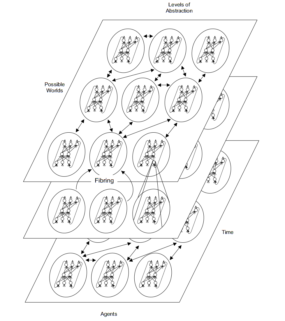
For example, speaking of the respected Hinton and his deep learning, we can imagine the neural network as fibring (fibring, stratification), when the subnets responsible for symbolic knowledge are recursively formed in each other. Imagine the variables X, Y, and Z and the two subnets responsible for the concepts of P (X, Y) and Q (Z). Then the meta network in fibring will map P and Q to the new concept R (X, Y, Z) so that P (X, Y) ^ Q (Z) -> R (X, Y, Z). Although practical implementation is very difficult. The cognitive model should handle complex relationships in the observed data (eg tactical maneuvers, safe driving). Unfortunately, a human expert often does this in a non-deterministic and subjective way (for example, based on stress or fatigue), and it is not quite clear how to convey this experience to the model.

Another example is the NSCA (Neural Symbolic Cognitive Agent) architecture, based on the Boltzmann Recurrent Temporal Limited Machine (RBM) from Sutzkever, Hinton and Taylor (2009). The two-layer RBM network receives some knowledge as temporal logic at the input, changing its weights, and calculating output weights by weights in response to input vectors is a probabilistic argument. Thus, the rules of temporal logic are given by RBM weights. The NSCA architecture was used in driving simulators, in the DARPA Mind's Eye project and in Visual Intelligence systems. Also in 2014, it was involved in automotive CO2 emission reduction systems. Now it is integrated with deep Boltzmann machines from Hinton and Salakhutdinov, although it is hinted that NSCA still has many unresolved problems.

Neurosymbolic systems originate in cognitive science and neuroscience. The first theory of human thinking was formulated by Johnson and Laird in 1983. Until now, the central problem is the neural binding mechanism (i.e., the binding problem). exactly how the isolated images fit together. For example, the theory of conjunctive codes (conjunctive codes) for neural binding is closest to existing artificial neural networks (ANN). According to this theory, for neurons in the brain there is no single binding resource (combinatorial explosion), but there are well-scaled distributed representations, moreover, they appear randomly and are effectively discriminated. However, neuroscience is largely rejected by modern ANNs to explain thinking, although they recognize their merits. So, since 1988, Fodor and Pylyshyn have argued that thinking is by its own nature, giving an interesting analogy to software and hardware. The functional complexity is in software, symbolic in nature, and any algorithm is determined by the software, and not by its representation in hardware. Further, modern experiments show that a person is inclined to use rules to solve cognitive tasks, and these rules are individual and correlate with IQ. In addition, there is a central executive function responsible for planning and localized in the frontal lobe. Further, among psycholinguists, there is still a debate about whether language morphology is based on rules or on associations. Finally, connectionism does not reflect the representative compositional nature of many cognitive abilities (Ivan in the sentence “Ivan loves Masha”! = Ivan in the sentence “Masha loves Ivan”). In the concept of modern ANNs, the aforementioned aspects are insoluble.

Logical reasoning in modern INS is presented as follows (see Pinkas and Lima, 1991-2013). Let's say that our task is a conclusion on a knowledge base in first-order logic, and take an ANN with a symmetric weights matrix (for example, RBM). Our knowledge base will be represented by weights or activation of any neurons. Then the INS conducts a gradient descent for the energy function, the global minimum of which is the conclusion in our chain of reasoning.

In the second part, examples of reasoning and first-order logical operations in the ANN, Markov's logical networks, examples of other approaches using LSTM, complexity and predictions for the future.

4. Overcoming catastrophic forgetting in neural networks

Authors: James Kirkpatrick, et. al. (DeepMind, Imperial College London, 2016)
→ Original article
Review author: Jan Sereda (in @ yane123 slake)

We made the assumption that not all network parameters are equally important for performance on the learned task A. We decided to modify the learning algorithm so that it would reveal the “important” weights for the already learned tasks and would protect them from a strong change - proportionally to the degree of their importance for the past learned tasks.

This was achieved by adding a penalty to the loss function. The penalty for changing a parameter (weight or bias) is proportional to the square of the change. The proportionality coefficient (that is, the indicator of the importance of the parameter for task A) is Fisher information, calculated for this parameter and the dataset of task A. First derivatives are sufficient for calculating the Fisher matrix.

If, after tasks A and B, we begin to teach the network to problem C, then the loss function, respectively, will be already out of three components (for damage A, for damage B, and for the quality of solution C).

They also suggested a way to measure the degree of re-use by the network of the same weights for solving different tasks - “Fisher overlap”.

Experiments: on synthetics, mnyste and atari

5. Deep Image Harmonization

Authors of the article: Yi-Hsuan Tsai, Xiaohui Shen, Zhe Lin, Kalyan Sunkavalli, Xin Lu, Ming-Hsuan Yang (University of California, Adobe, 2017)
→ Original article
Review author: Arseny Kravchenko (in @arsenyinfo slake)

If you cut an object from one picture and stupidly paste it onto another, it is easy to guess that it’s unclean - you’ll notice differences in light, shadows, etc. In order to disguise their activities, the masters of Photoshop twist some curves, but the DL guys have an alternative solution.

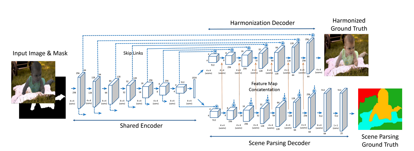
Let's teach the end-to-end network that will turn poorly photographed photos into almost real ones. The problem with the data: there are no classic X, Y pairs for supervised learning. But you can generate such data: take a picture from a dataset like COCO, select an object on it using a mask and “spoil” it - transfer color characteristics to it (for example, using histogram matching; however, the authors used many more advanced techniques). Since COCO is not diverse enough, let's do the same way distorted images from the flicker and filter (hello, #proj_kaggle_camera!) Too disgusting with the help of aesthetics prediction model.

Now you can learn the network encoder-decoder architecture: unet: turn distorted pictures + distortion masks into original ones using normal L2 loss. To further improve the quality, let's do multi-task learning: we will add a second decoder branch, which will be responsible for semantic segmentation, and, accordingly, we will add cross-entropy to the loss. The final architecture looks like this.

Pictures look really cool .

The authors laid out the model and weights on Caffe, but there is a fatal flaw - I personally could not lift the model (it seems that some fixed version of caffe is needed, but which one is not clear).

6. Accelerated Gradient Boosting

Authors: Gérard Biau, Benoît Cadre, Laurent Rouvìère (Sorbonne Université, Univ Rennes, 2018)
→ Original article
Review author: Artem Sobolev (in asobolev slake )

In optimization theory it is known that gradient descent is a rather slow procedure. There is a so-called Newton's method of correcting the direction of change of parameters using the Hessian matrix, but it is computationally more complicated and requires additional calculations. Of the first order methods, i.e. using only the gradient and the value of the function, the optimal (for a certain class of problems) in the rate of convergence is the fast gradient Nesterov method

This article proposes to insert this optimization method in the gradient boosting. Considered simple: the method converges faster, which means that such a fast gradient boosting should have better quality with fewer assembled models.

The authors conducted several experiments, comparing with the usual gradient boosting. The data was used strange: several synthetic datasets and five of them in the UCI repository. True, the authors show (Fig. 3) that fast gradient boosting learns much faster than usual, however, they show it on synthetic data. In general, according to the results of their experiments, the authors state that the method works no worse, is less sensitive to the learning rate, and uses fewer models in the ensemble.