Heading "We read articles for you." December 2017 - January 2018

Hi, Habr! We continue to publish reviews of research papers from members of the Open Data Science community from #article_essense. Want to get them before everyone else - join the community !

Articles for today:

1. LightGBM: A Highly Efficient Gradient Decision Tree Gradient Boosting (Microsoft Research, NIPS 2017)
2. Deep Watershed Transform for Instance Segmentation (University of Toronto, 2017)
3. Learning Transferable Architectures for Scalable Image Recognition (Google Brain, 2017)]
4. AdaBatch: Adaptive Batch Sizes for Training Deep Neural Networks (University of California & NVIDIA, 2017)
5. Density estimation using Real NVP (University of Montreal, Google Brain, ICLR 2017)
6. The Case for Learned Index Structures (MIT & Google, Inc., NIPS 2017)
7. Automatic Knee Osteoarthritis Diagnosis from Plain Radiographs: A Deep Learning-Based Approach (Nature Scientific Reports, 2017)

1. LightGBM: A Highly Efficient Gradient Boosting Decision Tree

Authors of the article: Guolin Ke et. al., Microsoft Research, NIPS 2017
→ Original article
Review author: Fyodor Shabashev (@ f.shabashev in slake)

LightGBM is positioning itself as a library for fast learning of boosting models and recently lightGBM developers published an article on NIPS that described two heuristics that help train boosting on trees faster. Both heuristics were implemented in lightGBM about 6 months ago.

1. Gradient-based One-Side Sampling (GOSS) - the heuristic is to sub-sample objects with small gradients at each step of the boosting. That is, the gradient on each object is considered, the objects are sorted in descending order of the absolute value of the gradient, then to build the next tree, only the top N objects with the largest gradient and the sub-samples of other objects are taken.
   According to the authors, this heuristic reduces the learning time by 2 times with a slight deterioration in the quality of the model.
   This heuristic is boosting setting the boosting parameter to goss . Github docs

   
   
2. Exclusive Feature Bundling (ERF) - the heuristic is to glue several sparse signs into one.
   Thus, even before building the first tree, several signs of the form are taken:

(1, 1, 0, 0, 0, 0)
(0, 0, 0, 1, 1, 0)
(0, 0, 0, 0, 0, 1)

and converted to one sign of the form:

(1, 1, 0, 2, 2, 3)

After such gluing, the calculation of the optimal split will go faster, as there will be less signs.
According to the authors, this heuristic also gives a significant acceleration on some datasets.
As far as I understand ERF is enabled by default. Github config Therefore, if there is no sparse feature in dataset, then it may be useful to turn it off.

2. Deep Watershed Transform for Instance Segmentation

Authors: Min Bai, Raquel Urtasun, University of Toronto, 2017
→ Original article
Review author: Vladimir Iglovikov (here and in ternaus slake )

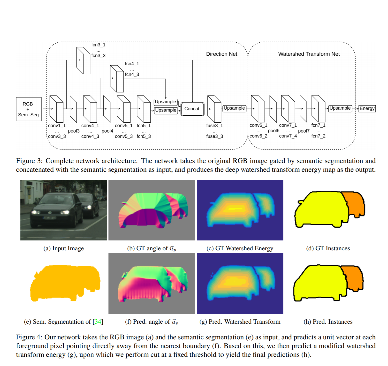
The article is trying to solve this problem: let us have pictures and it does not matter, grayscale, RGB, satellites, something else. And there are binary masks that distinguish some type of object, that is, the task of Semantic Segmentation has already been solved.

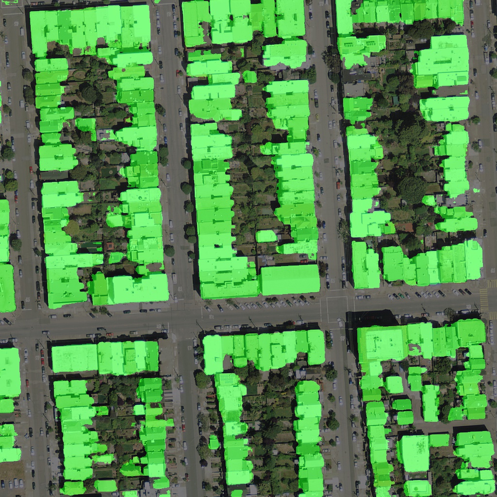
Now I want to cut the binary mask into separate objects. That is, to do exactly what the pressure on the winners of Urban3d ( albu , @selim_sef, Victor ) in many ways snatched the victory and money from the geese. Let there be such a prediction of houses in the satellite image (green - predicted mask)

The article proposes a framework that just allows you to apply the watershed transform, but in a more intelligent end2end Deep Learning mode.

So the steps they take:

1. The binary mask that we have is attached to the fourth channel at the entrance (you can probably do without it).
2. On the NxN binary mask, a vector field is created, where each pixel is associated with a unit vector, which is directed along the gradient from distance transform to the nearest border. Represented as a matrix (2xNxN)
3. A certain network is being trained (I think that the architecture can be improved 100,500 times, but this is not the point), which takes 4 channels as input (RGB + binary mask) and the output is calculated in paragraph 2
4. For each mask, a watershed transform is made and an energy level cutoff is located which allows the initial mask to beat on the instances.
5. A second network is being trained, which takes as input the item 2, that is, the output from item 3 and the output performs the classification, the purpose of which is to predict the binarized energy level from item 4.

In general, if in simple terms, the guys suggested a neural network way to implement the watershed transform binarization.

• and, it is they who did a great job, they did a submit on Instance Segmentation on CityScapes - there they have the sixth place on LB.

In prichinpe all this action, that is

• segmentation
• vector field prediction
  -prediction of energy level

can be assembled into one pipeline, and even arrange sharing of aggressive features (such as Faster RCNN, fell on Fast RCNN shoulders) and get a fairly strong and most likely smart model

3. Learning Transferable Architectures for Scalable Image Recognition

Article authors: Barret Zoph, Vijay Vasudevan, Jonathon Shlens, Quoc V. Le. Google Brain, 2017
→ Original article
Review author: Maxim Lashkevich (here BelerafonL , in Slake belerafon)

In general, they make meta-teachers to search for the most optimal architecture for image recognition: such as LSTM, they generate the architecture, they teach this architecture from scratch to recognize pictures, and use the accuracy received as a reward for the RL algorithm that teaches this very LSTM. And they got this same state-of-art on the imagenet.

In general, they say - it’s impossible to train such a thing on the imagemap right away, because in order for the RL algorithm to learn something there, you need tens of thousands of iterations, and even Google cannot afford this. Therefore, let's train on CIFAR-10, but now we need to somehow extend the result to the imagenet. But how to extend to another dataset the generated architecture, which is generally incomprehensible how it works and why exactly this one? In order to be able to do this, they impose certain limitations on the meta-teacher, so that he searches for the optimal architecture, but not any, but so that it consists of consecutive layers of the same type (Cell, Cell): Normal Cell, which is supposed to be a complicated replacement for the convolutional layer and should learn some features, and Reduction Cell, which should perform the reduction of dimension. And if such optimal cells are found on CIFAR, then for the image you can just infuse them a little more and that's it, the type should work fine too. And, oddly enough, it rolled, and it is - the figure shows how they drain these cells.

Exactly half of the article is occupied by benchmarks, as it all works out well. What everywhere means state-of-the-art results, and on the image, and on segmentation, and for mobile networks with small resources, and that both the accuracy is higher, and the computation of this generated network is less and the hair is curly. I will not give the results, who should look at their tablets, I’ll better tell you how the generator of this network works and what is there for.

This means that a simple single-layer LSTM of 100 neurons in a hidden layer is used as a generator. It receives nothing at the entrance (as I understood it), it just spits from the configuration of the architecture (or, more precisely, the configuration of Normal Cell and Reduction Cell, and they already flooded the manually specified number of times).

They generate the architecture of the cell in blocks (see picture): each block contains two inputs and one output (tensors).

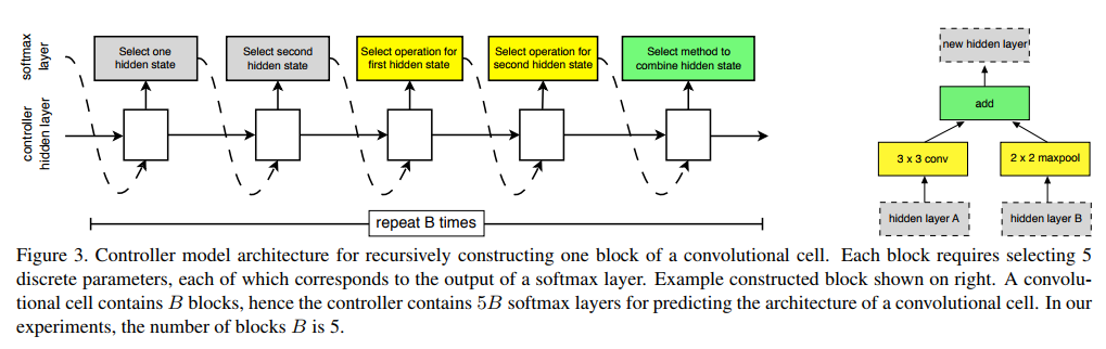
For each input, the generator can choose for some operation that it takes from a predefined set, which they selected empirically from the best traditions of building neural networks (the list next to the first picture), then the results of these two operations are combined into one tensor, which is also chosen by LSTM operation.

Here this operation can be either addition or concatenation. It turns out the unit has one way out. This output is added to the list of available "inputs" for the next block. And then the next block is generated. Thus, the generation process is as follows:

1. The first input is selected, with which we do something (for the first block it can be the output of the previous layer or the layer under it, or the input data, if it is the first layer). Those. LSTM issues softmax number, which input to take. And this is learning through RL.
2. Similarly, the second entrance is selected.
3. The operation is selected, what to do with input 1 (from the list of operations in the picture above)
4. The same for input 2.
5. The operation of combining the results of steps 3 and 4 is selected, and the resulting output is added to the pool of available inputs to generate the next block. Those. in points 1 and 2 for the next block, LSTM will select inputs from the list to which the output of the resulting block has already been added.

Thus, to generate a single block, LSTM spits five times. And they chose such blocks for each Cell ... also 5. Apparently, in order to confuse with that 5, which is the number of block generation steps. Therefore, to generate a single cell, LSTM is spat 25 times. And since both Normal Cell and Reduction Cell need to be generated, you need to spit two more times. They write this as a 2 × 5B formula, where B, the hyperparameter of the number of blocks, is 5.
So, the result of the best generated Cell is shown.

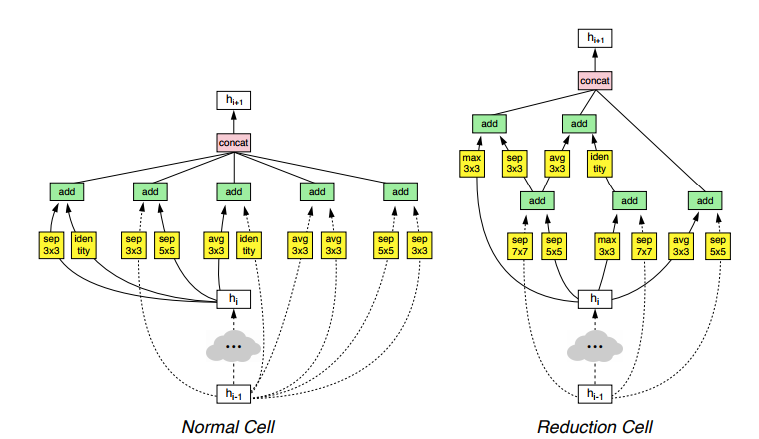
Why so? Ask LSTM, she knows better. But there are types of residual compounds, some blocks that are not typical for modern architectures, and nothing at all incomprehensible. But it works well for generally different networks in recognition and image segmentation. The main thing is to insist on the desired number of times. Interestingly, these are not the only good cells, and there are others that also work well, but visually inside are completely different (there are others in the app).

They also compare the teaching method. It’s debatable that RL teaches something better there than random search, and therefore they conducted experiments with bruteforce on the selection of architecture and showed that RL works better.

By the way, for RL they use Proximal Policy Optimization https://blog.openai.com/openai-baselines-ppo/ . They teach this stuff on a 500 (!) GPU, where almost all of them are slave workers who check the generated LSTM architectures. The number of iterations (trained neural networks on CIFAR) is tens of thousands.

Total.

1. The meta-learning algorithm itself turned out to be very simple. Compared to all sorts of alpha go there, there is one thin LSTM and that's it. No rocket ideas.
2. The idea in order not to generate the whole architecture, but to generate universal cells that can flow down, is undoubtedly excellent, and it took off.
3. The results on pattern recognition are afigenna, you can take and use the found cell architecture in your picture recognition projects, it should work.
4. It is not possible to repeat their results at home due to the need of the 500GPU, as well as, by the way, all other similar Google works.

4. AdaBatch: Adaptive Batch Sizes for Training Deep Neural Networks

Authors: A. Devarakonda, M. Naumov, and M. Garland, University of California & NVIDIA, 2017
→ Original article
Review author: Yegor Panfilov (in Slake egor .panfilov)

It so happened that when learning DNN, convergence is higher on small bats and better solutions are found. But only soon the Bitcoin bubble will burst, and a lot of crazy iron will appear on the market, which would be good to be able to dispose of for training in parallel (ie, to learn on large batch).

The authors propose a novel (lol) approach to AdaBatch, in which the size of a batch increases in the learning process adaptively. In a sense, this is equivalent to using learning rate decay, however, the authors show that both techniques can be used together.
The idea was tested on VGG, ResNet, AlexNet on datasets CIFAR-10, CIFAR-100, ImageNet. Compared with similar architectures, where batch size is fixed.
At one P100 on CIFAR-100 every 20 epochs used learning rate decay 0.75, and for the adaptive method they also increased the size of the batch by 2 times. As a result, the network with adaptive batch size gained the same quality as with a small, but direct and reverse pass, on average, took place 1.25, 1.15 and 1.46 times faster (respectively, in architecture).

The next experiment mixed 4 P100s and PyTorch.nn.DataParallel and overclocked to 1024-16384 batches (used lr warmup (technique from Facebook, if you remember) at the beginning, after - lr decay 0.5 and doubling the batch every 20 epochs). According to the results, they again achieved a quality similar to training with a fixed 128 batch, but 3.5 times faster for VGG19 and 6.2 times faster for ResNet-20.

We also wanted to measure on ImageNet, but the video cards ran out of memory on the 512 batch, and the authors decided to accumulate gradients (driving the batches one by one, and then using backprop). It is clear that the acceleration of training in this situation is difficult to measure, but you can compare the accuracy. AdaBatch with the initial batch in 4096 and the final 16384 again shows comparable results with training on a fixed 4096.

5. Density estimation using Real NVP

Authors of the article: Laurent Dinh, Jascha Sohl-Dickstein, Samy Bengio. University of Montreal & Google Brain, ICLR 2017
→ Original article
Review author: Arthur Chakhvadze (in @nopardon slake)

Sometimes you want to simulate complex distributions, from which you can simply get a sample and which can effectively calculate the density at a point. For example, such a problem arises when learning deep Bayesian networks, where the accuracy of the estimation of reasonableness depends on the flexibility of the variational distribution.

There are two main approaches to this task. Autoregression models such as MADE, NADE, PixelRNN, PixelCNN, and so on. decompose the joint distribution p (x1, x2, x3, ...) to the product of conditional p (x1) p (x2 | x1) p (x3 | x2, x1) ... They allow you to simulate very flexible families, but they do not scale well to high-dimensional data, since the complexity of sampling is proportional to the dimension of the random variable.

An alternative approach is based on the variable change formula: if a random variable z with density p (z) is transformed by some invertible function f, the density f (z) is p (z) / | det J |, where J is the Jacobian of f.
Normalizing flows use this fact to build complex distributions, applying a sequence of reversible functions to normally distributed noise. The main problem of the approach is that the calculation of the Jacobian in the general case requires O (n ^ 2) operations, which is unacceptable for high-dimensional data. The first proposed flows, planar and radial, have a very simple form and make it possible to calculate the determinant of the Jacobian clearly in linear time, however, to obtain a complex distribution, a very long chain of such transformations is needed.
Inverse Autoregressive Flows use mappings of the form z -> z + f (z), where f is a neural network with an autoregressive structure, that is, the output f (z) [i] depends only on z [j] with j <i. The Jacobian of such a transformation is a lower triangular matrix with units on the diagonal and its determinant is equal to one. In practice, unfortunately, it turns out that due to the autoregressive network structure, such transformations are not as effective as we would like.

The authors of the article suggest using a network consisting of “twin layers”. Each “double layer” transforms the n-dimensional input vector X into an n-dimensional vector Y reversibly. First, the elements of the vector X are divided into two sets - X_a and X_b. X_a is displayed unchanged to itself: Y_a = X_a. On the X_b layer acts as an affine transformation, the parameters of which are given by the part X_a: Y_b = X_b * exp (scale (X_a)) + shift (X_a), where scale and shift are arbitrary neural networks. The Jacobian of such a mapping has a block triangular structure, and the diagonal blocks are diagonal matrices. The proposed layers allow you to model very complex distributions (for example, the distribution of individuals) and do not require networks like MADE or PixelCNN as autoregressive functions.

Began to understand more, it turns out, the authors published an article with almost the same idea back in 2014. At the same time in the article about Normalizing Flows they write that the planar flow works better. Apparently, RealNVP / NICE begins to bend when the dimension is large and it is possible to exploit the structure in the data, for example, by convolutional networks.

As for the IAF, I had to pick MADE with a stick for a long time in order to get better than at least Housholder Flow, which is, in fact, linear.

And here RealNVP is used to parameterize the weights on the weights. It seems to work on mnyste.

6. The Case for Learned Index Structures

Authors: Tim Kraska, Alex Beutel, Ed H. Chi, Jeffrey Dean, Neoklis Polyzotis. MIT & Google, Inc., NIPS 2017
→ Original article
Review author: Evgeny Vasilyev (in evgenii .vasilev slake)

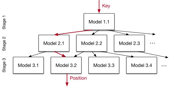
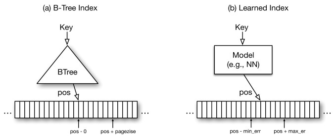
Approaches to data indexing have long been more or less settled down, but the guys from Google think that by shaking the neural network everything can be improved, and in this case it seems to work. Indexing data can in fact be reduced to an ML problem, there is an input - a key and you need to predict its location in a sorted table. At first they try to solve the problem head-on and feed it all to one network, but it turns out that it is expensive and not optimal than the B-Tree, with which they compare the model. Instead, they offer a “recursive regression model,” which in essence is a hierarchy of very simple neural networks. The upper layer takes the key and predicts that the models from the lower layer will give this key further to the prediction, while the lowest model already predicts the position in the table. This system can also be mixed with B-Tree, replacing the lowest models of the proposed recursive model, which predict the immediate position of the key in the table on B-Tree, which they believe should accelerate. They compared the different architectures of the B-Tree and the two-level recursive model. In their proposed model, the neuron architecture was selected by a griddle from 0-2 layers of 4-32 neurons. Benchmarks were made on three different datasets with sizes ranging from 10 to 200m, and the ML system was 3x faster and took up much less space. They also tried to compare the new system with the Hash table and Bloom's filter (checking the presence of the key in the table), where it turned out to be about the same speed as the classic models, but it took a little less space. The most interesting is that all the benchmarks were made on the CPU. The authors believe that with GPU / TPU, the possibilities for improvement are enormous and give a lot of ideas for further drawing. In general, I advise you to read the article, it is very well written.

7. Automatic Knee Osteoarthritis Diagnosis of Plain Radiographs: A Deep Learning-Based Approach

Authors of the article: Aleksei Tiulpin, Jérôme Thevenot, Esa Rahtu, Petri Lehenkari, Simo Saarakkala. Nature Scientific Reports 2017
→ Original article
Review author: Aleksei Tiulpin (in lext slake )

What's so special about the high impact of the magazine.

1. For the first time, the use of Siamese networks for images where there is symmetry was proposed. For example, these are joints, and it is obvious that it is better to fumble features from the left and right parts when learning and inference. Experiments have shown that it works better than not fumbling.
2. One of the first works where it was proposed to artificially limit the attention of the network, since it is very important that she look in the correct areas. GradCAM was also shown for the original network topology.
3. It is shown on examples from the clinical point of view that the method with a little less accuracy is better for doctors - they trust more what is interpreted easily.
4. SOTA performance
5. The code is open, which can not be said about other articles where they work with medical data.

In conclusion, I want to say that in medicine, boost in performance is not very important. The interpretability of the network is important. Moreover, it seems to me that finetuning doesn’t really go well in medical tasks and needs a little special approach.

, - . , , #article_essence. - — .