Smart face control: machine learning algorithms for efficient data caching on SSD

This article was presented at the SECR2017 conference, where it won the Bertrand Meyer award for the best research report.

In this material, Svetlana Lazareva, the head of the research laboratory “Radics”, talks about a new algorithm for filling a parallel cache in the storage system, which is based on a machine learning algorithm.


Original article and presentation .
')

Hybrid systems

The main customer requirements for storage systems are the high I / O performance provided by solid-state drives (SSD) and the low cost per operation guaranteed by disk drives (HDD). The reason for the differences between hard drives and solid-state drives lies in their internal work. HDD to access a specific data block is required to move the head and rotate the magnetic disks, which in the case of many random requests leads to high costs, while the SSD has no mechanical parts and can serve both sequential and random requests with the same high speed.

But the high performance of solid-state drives has reverse sides. Firstly, it is a limited service life. Secondly, this is the price, which per unit of capacity is noticeably higher than that of traditional HDDs. For this reason, data storage systems built exclusively from SSDs are of limited distribution and are used for particularly loaded systems that have expensive data access times.

Hybrid systems are a compromise between cheap but slow storage on HDD and productive, but expensive storage on SSD. In such systems, solid-state drives play the role of additional cache (in addition to RAM) or tiring. In this article, we gave arguments on the choice of a particular technology.

Using solid-state drives as cache devices in combination with a limited number of rewriting cycles can significantly speed up their wear due to the logic of traditional caching algorithms leading to intensive use of the cache. Thus, hybrid storage systems require special caching algorithms, taking into account the features of the used cache device - SSD.

The simplest implementation of the idea of ​​a hybrid array is a second-level cache (see Figure 1), when all requests after the RAM are on the SSD. The basis of this approach is the property of temporal locality - the probability of requesting the same data is the higher, the smaller the last access time. Thus, using SSD-cache, as a second-level cache, we would increase the amount of RAM. But if the RAM is enough to handle temporary locality, then this method is not effective. Another approach is to use SSD cache as a parallel (see Figure 2). Those. some requests go into RAM, some immediately into the SSD cache. This is a more complex solution, aimed at the fact that different caches handle different locality. And one of the most important moments of the implementation of the parallel level cache is the choice of SSD cache filling technique. This article describes a new algorithm for filling a parallel cache — face control, based on a machine learning algorithm.

The proposed solution is based on the use of data from the history of requests to storage systems recorded over long periods of time. The decision is based on two hypotheses:

• Query histories describe typical storage load for at least a limited amount of time.
• Storage load retains some kind of internal structure that determines which blocks and with what frequency are requested.

While the first hypothesis is almost beyond doubt and remains an assumption, the second requires experimental verification.


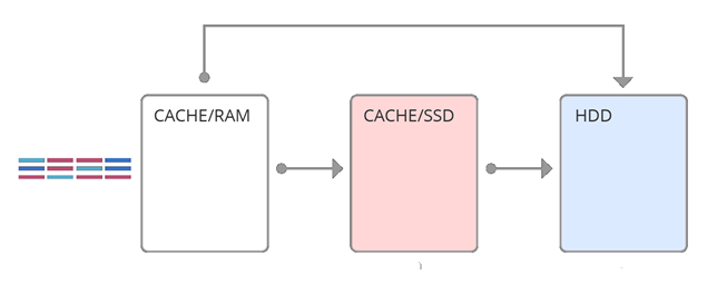
Fig. 1. Second Level Cache


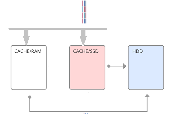
Fig. 2. Parallel cache

Solution Architecture

The architecture of the proposed solution is presented in Fig. 3. All requests coming from customers, first go through the analyzer. Its function is to detect sets of consecutive requests to the system.


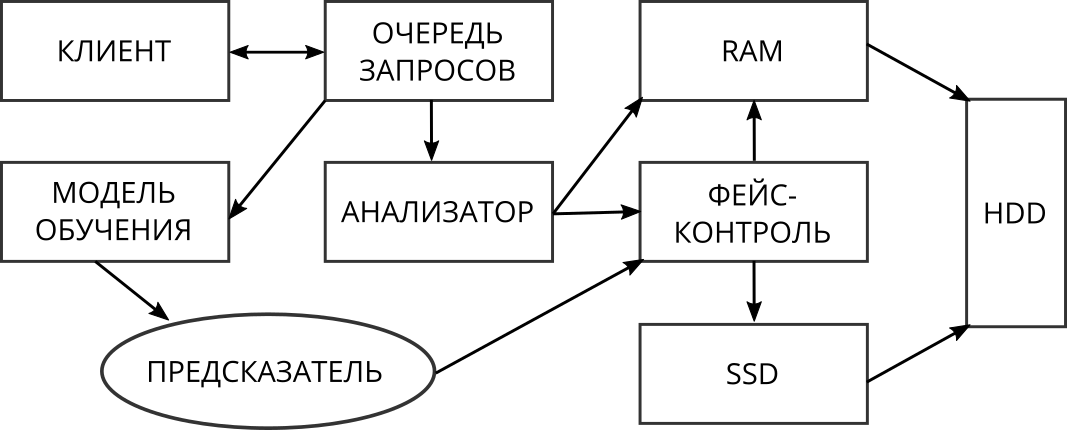
Fig. 3. Solution architecture

Depending on the type, they are processed differently:

• Sequential write Requests of this type do not cause problems and are processed quickly, so the data they are accessing does not fall into the SSD cache.
• Sequential reading . Requests of this type are processed quickly due to read-ahead algorithms, usually such requests are unique (ie, repeated sequential reading of the same data is unlikely), so such data is not necessary to be cached in the SSD.
• Random entry . Such requests cause noticeable costs in both write-through and when injected into RAM, since data when popping out of the cache will still require writing to hard drives. Therefore, they immediately, bypassing the RAM, are sent to the SSD cache for writing, where they are stored log-structured and pushed out as consistently as possible for more efficient further writing to the array of hard drives.
• Random reading . Data is cached in RAM or in SSD depending on the face control algorithm.

In this system, only random queries affect SSD wear. Random write requests cannot be optimized. Thus, the only way to increase the life of an SSD is to optimize the processing of requests such as random reading. If you have a way to assess the potential effect of caching specific data, you can get rid of the need to cache “unnecessary” data.

Works that offer solutions to increase the service life of SSD in hybrid storage systems as a whole can be divided into two groups. The first group considers the possibility of improving the efficiency of caching based on solid-state drives through the use of internal logic and technical features [5, 1]. Such algorithms are highly dependent on the specifics of specific devices and therefore will not be further illuminated.

The works of the second group focus their attention on creating new caching algorithms. The idea of ​​all is common: rarely used data should not fall into the cache. This, firstly, reduces the number of entries in comparison with traditional algorithms and, secondly, increases the number of cache hits due to less clogging of the cache with few used blocks.

• LARC - Lazy Adaptive Replacement Cache [4]. The algorithm uses simple logic: if a block was requested at least twice in a certain period of time, then it will probably be needed in the future and will be included in the SSD cache. Candidate blocks are tracked using an additional LRU queue in memory. The advantages of this algorithm include relatively low resource requirements.
• WEC - Write-Efficient Caching Algorithm [6]. Standard caching algorithms do not allow frequently used blocks to be continuously in the cache. This algorithm is designed to allocate such blocks and ensure that the cache is in the cache for the time of active access to them. This work also uses an additional cache queue, but with a more complex logic for determining candidate blocks.
• Elastic Queue [2]. Indicates a lack of all previously proposed caching algorithms: lack of adaptability to different loads. It considers the work with the priority queue as a common basis, and the differences in the logic of assigning priorities and suggests a generalized improvement in the queue from this point of view.

At the root of the algorithms discussed above, there is a natural method in computer science - the development of algorithms, often of a heuristic nature, based on an analysis of existing conditions and assumptions. This paper offers a fundamentally different approach, based on the fact that the workload to the storage system is self-similar. Those. By analyzing past queries, we can predict future behavior.

Machine learning algorithms

This task can be approached from two sides: using traditional methods of machine learning or representational learning. The former first require data processing to extract relevant features from them, which are then used to train models. Methods of the second approach can directly use the initial data that underwent minimal preprocessing. But, as a rule, these methods are more complex.

An example of a presentation training can serve as deep neural networks (see [3] for more details). As a simple base model, you can try decision trees. Signs on which training will be performed can be:

• Mean Time Stack Time
• The ratio of the number of reads and records
• The ratio of the number of random and sequential queries that are calculated on fixed segments of the query history.

The presentation teaching methods are promising. The available data are time series, which can be considered when choosing the appropriate algorithms. The only group of algorithms that use the information about the sequential data structure in their calculations is recurrent neural networks [3]. Therefore, models of this type are the main candidates for solving the problem.

Data

Data is a history of queries to the storage system. The following information is known about each request:

• The time of the request;
• The logical address of the first block (logical block address - lba);
• Request size (len);
• Type of request - write or read;
• Type of request - sequential or random.

Experiments and data analysis were carried out on real loads received from different customers. The file with the history of requests from customers in the future we call the log.
To analyze the effectiveness of a particular caching algorithm, you must enter a metric. Standard metrics such as the number of cache hits and the average access time to the data are not suitable, because they do not take into account the intensity of use of the cache device. Therefore, we will use Write Efficiency [6,2] as a metric of caching efficiency:

$$

$$WE = \ frac {number \: hits \: to \: cache} {number \: records \: to \: cache}$$

Query history is divided into blocks of successive queries. Block size is denoted as blocksize. For one query, the metric is calculated as follows: history looks for the closest windowsize queries and counts the number of queries to the same data as in the original. For a block of request blocksize, the average value of the metric by block is calculated.

Then the blocks are divided into two classes: “good” and “bad” (see Fig. 4). “Bad” (red) means that it is not recommended to send a block of requests to the SSD cache (it is sent to the RAM), “good” (green), respectively, that this block of requests is sent to the SSD cache. Those blocks whose coefficient WE is greater than the parameter m will be considered “good”. The remaining blocks will be considered "bad."


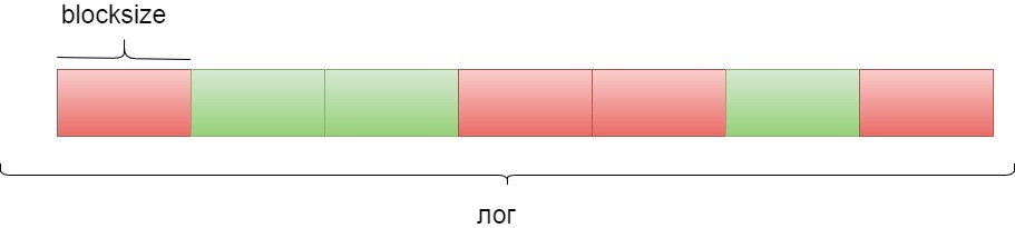
Fig. 4. Break logs into blocks

Calculating metrics for large windowsize values ​​can take a significant amount of time. Computational constraints are imposed on how far a block reuse can be calculated. Two questions arise:

• How to choose the windowsize option?
• Is reuse of blocks within windowsize a representative value for judging reuse of these blocks in general?

To answer them, the following experiment was conducted:

1. A random sample of requests was taken;
2. It is estimated reuse of these blocks within the significantly larger windowsizemax;
3. The Pearson correlation coefficient between the reuse of blocks within windowsizemax and windowsize is calculated, where windowsize is the different test values.

In fig. 5 shows the change in the correlation coefficient on the sample over time. Table 1 presents the value of the correlation coefficient for the entire sample. The result is significant (P-value is close to zero). It can be interpreted as follows: blocks that are in demand in the next windowsize requests are also likely to be in demand in the next windowsizemax requests.


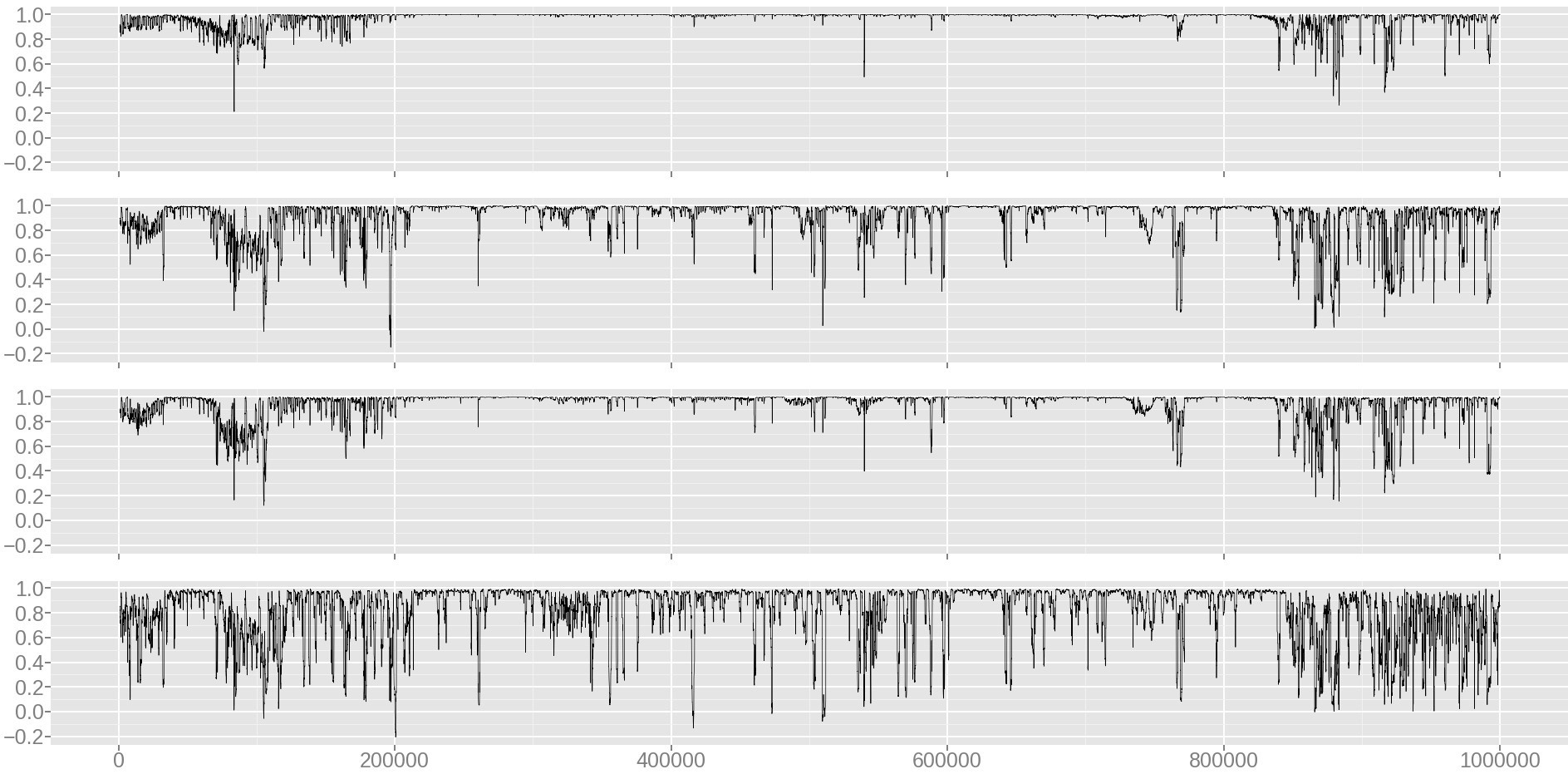
Fig. 5. Dynamics of the correlation coefficient between windowsize and windowsizemax
Comment to fig. 5. From top to bottom, windowsize: 100000, 10000, 30000, 3000. Sample size: 1,000,000 queries. The x-axis: the number of the running window of 1000 queries; y-axis: correlation coefficient value for a running window.

Table 1. Pearson correlation coefficient for different windowsize.

windowsize	3000	10,000	30,000	100,000
1,000,000	0.39	0.61	0.82	0.87

Thus, to calculate the metric, a windowsize value of 100000 is taken.
To build probabilistic models, the data set is standard [3, p. 120] was divided into three parts:

• Training sample: 80%;
• Test sample: 10% (for the final testing of the model);
• Validation Sample: 10% (for selecting parameters and tracking the progress of the model during training, regardless of the training sample).

It is worth noting that in the case of models of deep learning, samples cannot be made random, since in such a case the temporary connections between requests will be destroyed.

Deep learning models

Building a deep learning model requires multiple decisions. Provide a detailed explanation of each of them in this work is not possible. Some of them are selected according to the recommendations in the literature [3] and original articles. You can find detailed motivation and explanations in them.

Common parameters:

• The objective function is cross-entropy (the standard choice for the classification problem) [3+, p. 75];
• Optimization algorithm - Adam [7];
• The parameter initialization method is Glorot [8];
• The regularization method is Dropout [9] with the parameter 0.5.

Parameters tested:

• The number of recurrent layers of the neural network: 2, 3, 4;
• The number of output neurons in each lstm unit: 256, 512;
• The number of time steps of the recurrent neural network: 50,100;
• Block size (the number of requests in the block): 100, 300, 1000.

Basic deep learning method - LSTM RNN

It was tested models of varying complexity. For all, the result is negative. The learning dynamics is shown in Fig. 6


Figure 6. LSTM RNN. Change in loss function during training

Comment to fig. 6. Red - training sample, green - test. Graph for the model of medium complexity with three recurrent layers.

Pre-training and LSTM RNN

Pre-training was tested on the query flow modeling problem (prediction of the next query). The mean square error between the predicted value of lba and the present was used as the objective function. The result is negative: the learning process on the secondary task does not converge. The learning dynamics is shown in Fig. 7


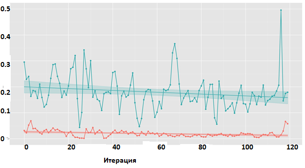
Figure 7. Pre-training on the lba prediction problem of the next query. Change in mean square error over the course of training.
Comment to fig. 7. Red - training sample, green - test. Graph for model with two recurrent layers.

HRNN

Were tested models for different sets of parameters, with two levels: the first for each block, the second for multiple blocks. The result of the experiment is negative. The learning dynamics is shown in Fig. eight.


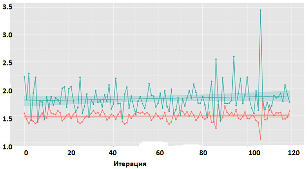
Figure 8. HRNN. Change in loss function value during training.

Comment to fig. 8. Red - training sample, green - test. Graph for the model of medium complexity with two recurrent layers at the second level.

As you can see, the neural networks did not give good results. And we decided to try the traditional methods of machine learning.

Traditional methods of machine learning. Attributes and signs.

Frequency characteristics and derivatives of them

We introduce the following notation:

• count_lba - the number of lba uses within a block;
• count_diff_lba - the frequency of the difference between the lba of the current query and the previous one;
• count_len - frequency of requests to blocks of a given length len;
• count_diff_len is the frequency of the differences between len current and previous queries.

Further, statistics are calculated for each attribute: moments: mean, standard deviation, coefficient of asymmetry, and coefficient of kurtosis.

Difference Characteristics and Derivatives from them

The difference between the lba of the current and the i-preceding block (let's call it diff_lba_i) can serve as the basis of the new feature. Each such diff_lba_i difference is symmetrically distributed and has an average equal to zero. Therefore, the differences between the diff_lba_i distributions for different i can be described using the singular, the standard deviation of this quantity. Thus, for each block, a set of n std_diff_lba_i values ​​is obtained, where i = 1..10 (we call this set lba_interdiffs). The hypothesis is that for good blocks of requests these values ​​will differ less, in other words, they will be more concentrated than for bad blocks. The concentration of values ​​can be characterized using the mean and standard deviation. The differences between them can be seen in Fig. 9.10, which shows that the hypothesis is confirmed.

Similarly, signs are calculated for the lengths of the requested data.


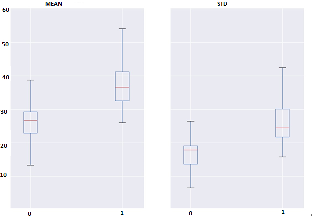
Fig. 9. Differences for classes between mean and standard deviations of the count_lba characteristic


Fig. 10. Differences for classes between mean and standard deviations of the lba_interdiffs feature

Feature analysis

To analyze the differences between classes with respect to signs, we plotted boxplots. For example, in fig. 9. Differences 1 and 2 moments of the count_lba feature are displayed, and in fig. 10 shows the differences between 1 and 2 points of the lba_interdiffs feature between classes.

The span diagrams show that not a single sign shows sufficiently significant differences between the classes to be determined only on its basis. At the same time, a combination of weak non-correlated signs may allow one to distinguish between classes of blocks.

It is important to note that when calculating signs, it is required to take a large value of the blocksize parameter, since in small blocks of requests many signs turn to zero.

Decision tree ensembles

An example of traditional methods of machine learning are ensembles of decision trees. One of its effective implementations is the XGBoost library [10], which has performed well in many data analysis contests.

The dynamics of the learning process can be observed in Fig. 11. On the test sample, a classification error of about 3.2% is achieved. In fig. 12 you can see the forecast model on the test sample.


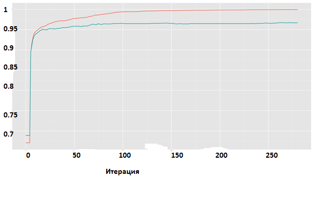
Fig. 11. XGBoost. Changing the classification accuracy during training. Red - training sample, green - test.


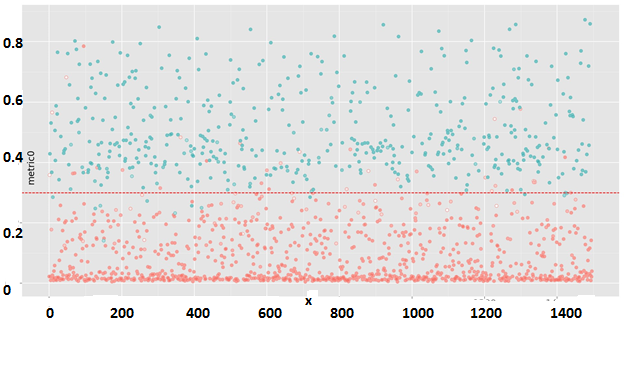
Figure 12. XGBoost. Prediction of the model on a random test sample
Comment to fig. 12. The color indicates the forecast model: red - poorly cached block, green - well cachable. The degree of color saturation is the probability derived by the model. X axis: the block number in the test set, y axis: the initial value of the metric. The dotted line is the barrier of the metric, according to which the blocks were divided into two classes for teaching the model. Error classification 3.2%.

Errors of one kind

In the task of caching, it is important not to make mistakes of the first kind, that is, false positive predictions. In other words, it is better to skip a block suitable for caching than to write to the cache.

unclaimed data. To balance the likelihood of producing false positive and false negative forecasts, you can change the probability barrier, after which the forecast will be considered positive. The dependence of these values ​​is shown in Fig. 13.


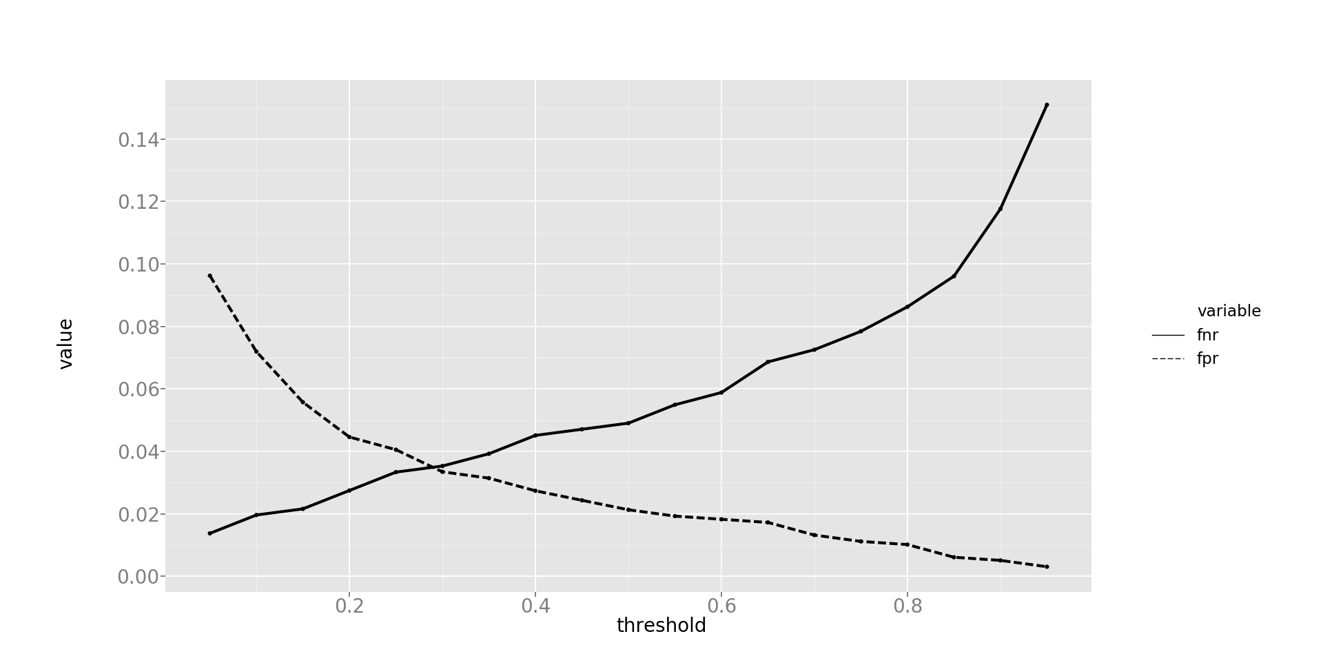
Fig. 13. Dependence of the probability of issuing false positive and false negative forecasts depending on the probability barrier, after which the forecast is considered positive.

Comment to fig. 13. The x-axis: the probability barrier, the y-axis: the probability of an error. The dashed line is the probability of making a false positive error, the solid line is the probability of making a false negative error.

The final algorithm is face control.

We describe the final algorithm describing the SSD cache filling technique. It consists of three parts: an algorithm that forms a training set of client logs, an algorithm that generates a prediction model (algorithm 2), and a final online algorithm that classifies incoming blocks of requests for “good” and “bad”.

Algorithm 1. Formation of a training set

1. The available sample is divided into blocks of size blocksize.
2. For each block we consider the signs from clauses 3.3.1 and 3.3.2.
3. For each block we consider the coefficient WE.
4. For each block, using the coefficient WE, we determine the class of the block: bad or good.
5. We make pairs (signs - class). For the characteristics of one block, the class of the next block is assigned.

Algorithm 2. Teacher

Input: list (signs-class) from algorithm 1.
Main loop: XGBoost algorithm.
Exit: predictor.

Algorithm. Face control

Input: block of length request blocksize, m.
Main loop: predictor from the teacher-algorithm.
Output: If the block is defined as good, then the next block of requests goes to the SSD. If the block is determined to be bad, then the next block of requests goes to RAM. If it was not possible to determine, then the requests from the next block go to the SSD if their frequency is greater than one (using the LRU method of the LARC algorithm).

Algorithm versus face control and popular SSD cache implementations

The face control algorithm was tested in a mathematical model, where it was compared with known implementations of the SSD cache. The results are presented in Table 2. In the RAM, the LRU displacement algorithm is everywhere. In the SSD cache of the LRU, LRFU, LARC displacement technique. Hits is the number of hits in the millions. The face control was implemented together with the LRFU crowding technique; it showed the best results in conjunction with the face control.

As we can see, the implementation of face control significantly reduces the number of records on the SSD, thereby increasing the service life of the solid-state drive and, according to the WE metric, the face-control algorithm is the most effective.

Table 2. Comparison of various implementations of SSD Cache

	Lru	LRFU	LARC	Face control + LRFU
RAM hits	37	37	37	36.4
RRC hits	8.9	eight	8.2	eight
HDD hits	123.4	124.3	124.1	124.9
SSD writes	10.8	12.1	3.1	1.8
WE	0.8	0.66	2.64	4.44

Conclusion

Hybrid storage systems are in high demand on the market due to the optimal price of 1 gigabyte. Higher performance is achieved through the use of solid-state drives as a buffer.

But SSDs have a limited number of records - overwrites, so using standard techniques to implement the buffer is not economically viable, see Table 2, since SSDs wear out quickly and need to be replaced.

The proposed algorithm increases the service life of SSD 6 times compared with the simplest LRU technology.

The face control analyzes incoming requests using machine learning methods and does not allow “unnecessary” data to the SSD cache, thereby improving the caching efficiency metric several times.

In the future, it is planned to optimize the parameter blocksize and improve the crowding technique, as well as to try other combinations of the crowding technique in the SSD cache and RAM.

Bibliography

1. Cache storage hybrid storage systems. / Yongseok Oh, Jongmoo Choi, Donghee Lee, Sam H Noh // FAST. –– Vol. 12. –– 2012.
2. Elastic Queue: A Universal SSD Lifetime Extension Plug-in for Cache Replacement Algorithms / Yushi Liang, Yunpeng Chai, Ning Bao et al. // Proceedings of the 9th ACM International on Systems and Storage Conference / ACM. –– 2016. –– P. 5.
3. Goodfellow Ian, Bengio Yoshua, Courville Aaron. Deep Learning. –– 2016. –– Book in preparation for MIT Press. URL
4. Improving flash-based disk cache with lazy adaptive replacement / Sai Huang, Qingsong Wei, Dan Feng et al. // ACM Transactions on Storage (TOS). –– 2016. –– Vol. 12, no. 2. –– P. 8.
5. Kgil Taeho, Roberts David, Mudge Trevor. Improving NAND flash based disk caches // Computer Architecture, 2008. ISCA'08. 35th International Symposium on / IEEE. –– 2008. –– P. 327–338.
6. WEC: Improving Durability of SSD Cache Drivers by Caching Write Efficient Data / Yunpeng Chai, Zhihui Du, Xiao Qin, David A Bader // IEEE Transactions on Computers. –– 2015. –– Vol. 64, no. 11. –– P. 3304– 3316.
7. Kingma Diederik, Ba Jimmy. Adam: A method for stochastic optimization // arXiv preprint arXiv: 1412.6980. –– 2014.
8. Glorot Xavier, Bengio Yoshua. Understanding the difficulty of training deep feedforward neural networks. // Aistats. –– Vol. 9. –– 2010. –– P. 249–256.
9. Graves Alex. Supervised sequence labeling // Supervised Sequence Labeling with Recurrent Neural Networks. –– Springer, 2012. –– P. 5– 13.
10. Chen Tianqi, Guestrin Carlos. XGBoost: A Scalable Tree Boosting System // CoRR. –– 2016. –– Vol. abs / 1603.02754. –– URL