Pumping C # Performance with Federico Luis
Today we will talk about performance in C #, about how to pump it beyond recognition. The goal of this article is to demonstrate ways to increase productivity, which, if necessary, you could use yourself. However, these techniques are not universal - you can not use them as a general solution to any problem. They are good in the presence of very specific use cases, which will be discussed below.
The report of Federico Luiz, the founder of Corvalius (they are involved in R & D) was chosen as a prototype of the article. Working on a database engine for one of the clients, they devoted about four years to optimization problems. This amount of time is required in order to apply all sorts of techniques and achieve good optimization indicators. It is required to identify all the problems and bottlenecks, to trace the behavior of the software in accordance with all available metrics and so on. The examples in this article are based on the work on RavenDB 4.0 (the well-known NoSQL base for .NET), which Federico Tyunil’s company is down to the nanosecond level in all sorts of complex cases.
All the examples that you will encounter during the story (plus some additional ones) are available in a special repository on GitHub .
Caution traffic! In this post there is a huge number of pictures - slides and screenshots from a video in 720p format. On the slides there is an important code for understanding the article.
A bit of math
Imagine that you came back from the next DotNext or Habra was reported during working hours, and your boss, believing that you were pumping high-quality in terms of performance, suggests developing a system that would perform 20 billion operations per day. Think about this number! Obviously, the idea is crazy - to realize unreal However, let's try to dig deeper and understand one important thing: 20 billion operations must be performed within 24 hours of continuous node operation . High or not, but our productivity will necessarily be sustainable. This fact allows us to go to other numbers: 20000000000/24 = 833333333 operations per hour. Is it easier for us? No, really. But we can continue to break our indicator further. We get that the required number of operations per minute: 833333333/60 = 13888888. Such a number is more or less amenable to counting. In the next step, we get the number of operations per second - 13888888/60 = 231481. In practice, the further solution of the problem is usually very simple: we take, say, 40 servers, each of which would have a performance of 231481/40 = 5787 operations per second . Better yet, if we take 1500 servers with a capacity of 231481/1500 = 154 operations per second. With these figures you can already work. It turns out that the number that initially seemed incredibly large to us no longer produces such horror. A single node and as many as 5 milliseconds of its operation will be provided for performing one operation. Moreover, in this case, we can confidently talk about the speed of our system. For comparison, computer games are released to the market with a mark of 13 milliseconds.
Order of numbers
Most high-performance systems sold are characterized by the ability of a single node to process about 600 requests per second in continuous mode. How is this possible? Of course, the indicator largely depends on the benchmark that is presented to the system: do we simply perform a series of repetitive operations that return the same thing each time, or do we send messages all over the world and generally know what? But the fact is that if our goal is to ensure that the node executes 600 requests per second in continuous mode, then in the initial design of the system we must lay the indicator 10 times larger and focus on it. And 6000 requests is a task that requires a different kind of effort from an engineering point of view. 6000 operations per second - an indicator that requires planning. It is necessary that someone constantly monitors the new code, which is added to the code base, and does not miss anything that puts the figure in 6000 operations at risk. And ultimately you will achieve this goal. But in order to achieve a performance that would be higher not by one, but by two orders of magnitude, that is, 60,000 operations per second, the same techniques will no longer work. Here we will need serious sophistication. Today I would like to share with you the secrets that we use in our work.
We will not discuss, but we take for axioms
- Interop is a constant source of resource overhead:
- Performance kills high marshaling frequency;
- Garbage collection is a major source of performance problems;
- You cannot use try-catch and LINQ:
- Epilogue and prologue for exceptions - not free;
- Calls to LINQ methods lead to memory allocation;
- With a high frequency of short operations, everything was gone;
- Any access to values via interfaces leads to heap memory allocation (in other words, there will be boxing;
- Value types need to be optimized in a special way;
unsafeis called unsafe for a reason;- GC pinning (explicitly blocking objects, prohibiting their movement in the memory by the garbage collector) is very expensive.
Everything you need to know about inlining
- Compiler directives are nothing more than hints;
- By applying inline, we reduce:
- the number of instruction cache misses;
- the number of Push / Pop operations and parameter processing;
- the number of context switches at the processor level;
- By applying inline, we increase:
- the size (in bytes) of the calling function;
- the locality of the link;
- Related effects:
- Dead Code Elimination;
- Constant propagation;
- The code can speed up or slow down (you need to measure everything!).
Even knowing all this, you can still find optimizing solutions. What comes next is completely based on our work experience. No publications, reports about this you will not find. Conclusions made by us rather empirically, based on our own observations.
Ordinal evaluation and Pareto-classification of bottlenecks
The famous Pareto law tells us that 20% of the code uses 80% of the resources. The assessment, we believe, is quite realistic. Raise this proportion to the square and scale down the values 100 times. We get the square of the Pareto law: 4.0% of the code uses 64% (about ⅔) of resources. If we raise the proportion to a cube and scale down 10,000 times, we get the Pareto law cube: 0.8% of the code uses approximately 51% (about half) of the resources. That is, having a code base of 1 million lines, we are forced to devote about half of the resources to the execution of only 5,000 lines. Pareto's law of the first, second and third order - this is what will help us to classify optimization techniques. We will conduct the favorite work of the programmer and decompose our technology into groups:
- In the first group we will place the optimization techniques working according to the Pareto law of the first order. These are techniques about the system architecture, network environment, ordinal complexity of the algorithms used (for the time being in terms of “big O”).
- The second group will go technology, for which the Pareto II order law is applicable. They involve work on optimizing the execution time of the algorithms. Is it possible, for example, to prevent the repeated execution of the algorithm that can be executed only once?
- The third group is Pareto's law of the third order, and here we are confronted with truly complex things that require real ingenuity. These are the so-called micro-optimization techniques.
I must say that, as a rule, the initial performance of your system will require the use of techniques of the first group. If the level of system optimization is below a certain threshold value, then it is too early for you to think about the techniques of the second and third groups.
Working on RavenDB
Now I will show you the problems that we dealt with when working on the RavenDB product a couple of versions ago. RavenDB is a fully managed document-oriented database. In the days of RavenDB 2.0, we used Microsoft ESE storage (also known as Esent). The product is good. But a problem soon emerged: each time a data was saved, the interop call was made, which, as we know, is quite resource-intensive. Other performance problems arose, in part, due to the use of cryptographic hashing, due to JSON processing. We also performed insufficient batching and lost productivity using Write Locks when writing data. So, we decided to optimize the code base of RavenDB 2.0. We created our own repository, which was designed to solve the problem with interopes. And well, in return we got two new holes! In the same way, we discovered new problems after we optimized JSON processing and began to perform more batching. Removing existing bottlenecks, we received in exchange more and more new. But by that time, the actions we took gave a tenfold increase in performance on the critical branches of the code, which in itself is quite significant.
On the way from version 3.0 to version 4.0 of RavenDB, we decided to use a radically different approach - “Performance first”. We put customer requirements on the back burner, and put performance at the forefront. We began to work with local memory allocation, created our own string type. To avoid copying data and achieve full control over memory, we created our own binary serialization format. We developed our own compression algorithms, sharpened specifically for the types of stored data. We also made efforts to ensure full control of access to IO and memory (for example, it was necessary to be able to directly tell the kernel which pages to unload and load). It was extremely important to try to clear the code from virtual calls. It is impossible to judge the effectiveness of such methods beforehand, they are only evaluated in practice. And each successful optimization is not just a quantity, it is a new multiplier in the formula. Increased productivity is always its multiplication. Of all the botlneks that were present in RavenDB 3.0, I would like to consider three with you:
- JSON handling problem;
- memory management problems;
- a large number of virtual calls.
Work with memory
One way or another, we deal with requests all the time. The request begins and ends in some way. Memory allocation is also a request. First, the memory must be provided, and after use it must be returned. As our practice has shown, approximately 90% of cases memory allocation occurs for strings (such is the specificity of databases, because they mostly store strings). Then, in descending order, there are collections, Gen0 generation objects that fall under garbage collection (the so-called “fire & forget” objects), asynchronous operations, Context objects of lambda functions. If you are developing high-performance software, you will have to give up using the garbage collector. This means that you will also release the memory manually. We created such lines that we would manage not the environment, but we personally (literally referring to the disk). For brevity, we will call such strings "unmanaged."
Now we will deal with questions like: who owns this or that section of memory, how quickly can memory be allocated, is it possible to ensure high speed memory allocation, if it is a short line? If during the work we need (within the framework of the same thread) to perform another memory request, then, since the free segment will be located next to the ones already used, it will most likely be already loaded into the cache. But the presence of a botnek in your code may not give you the opportunity to conduct such jewelry work. In order for you to successfully engage in this kind of optimization, your code must be tailored sufficiently sparingly. However, this approach refers to the methods of the Pareto I order law, as it permeates the entire system architecture. Deciding on such transformations is usually not easy. You must be prepared to practically start from scratch. Your versions will not have binary software compatibility, which is problematic.
Anatomy of a ByteString
What is a ByteString ? Its implementation looks like this:
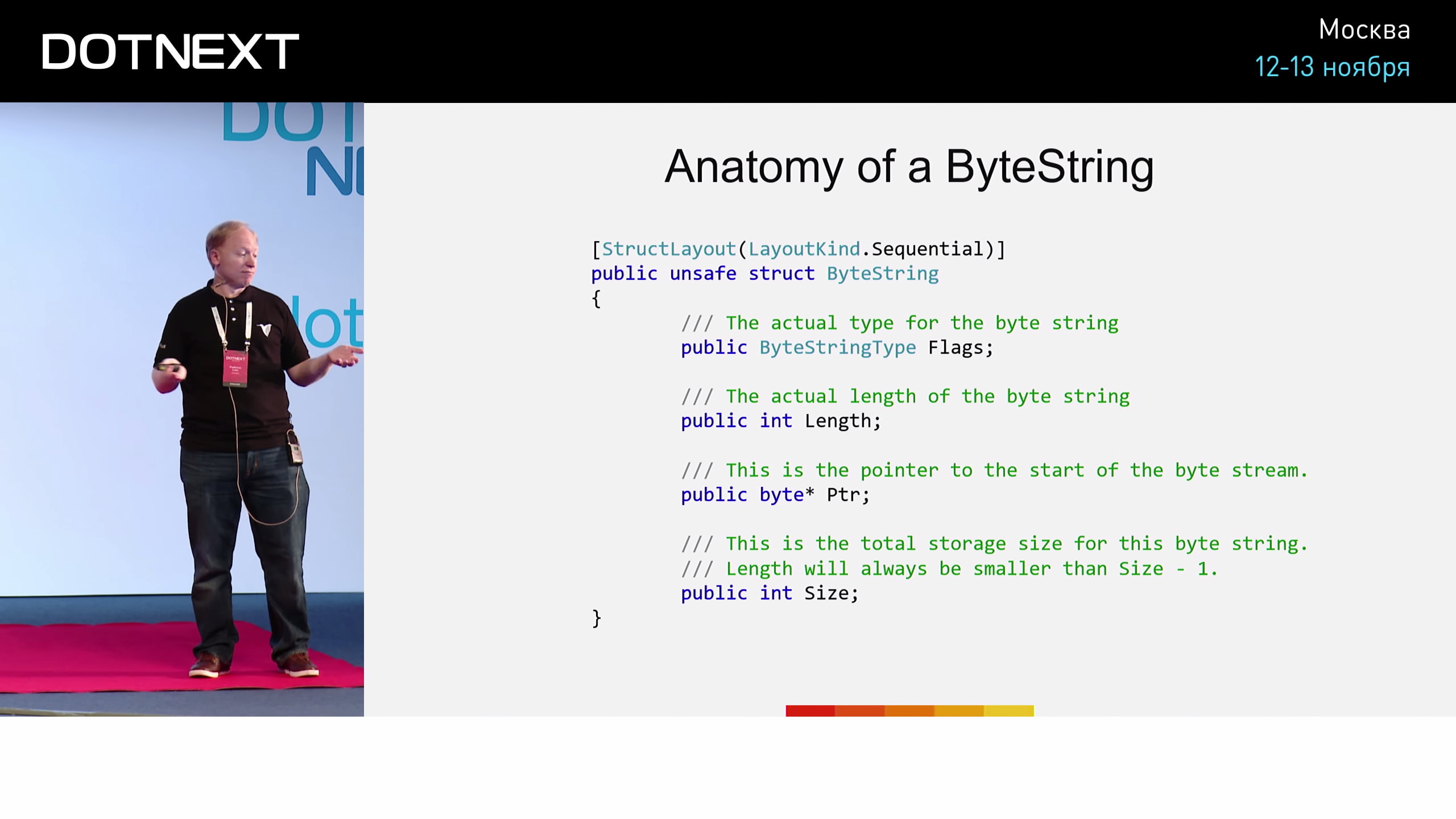
Several flags, the length of a ByteString , a pointer to the memory segment in which it is stored, as well as the size of this segment (in case we decide to release it with the possibility of someone else reusing it). Not much different from string type pluses, right? This implementation of ByteString reminds us of something else - the Span of the CoreCLR library.
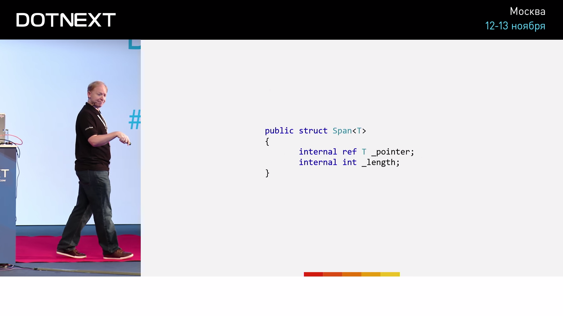
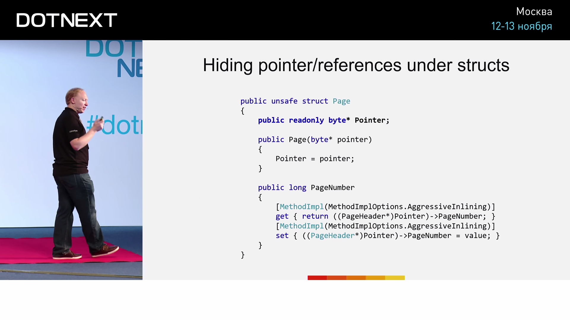
Span was first introduced in early 2016, and now entered the mainstream. Inside itself, Span stores a reference to a type. And what is the link? This is nothing but a pointer, carefully hidden from us for its beautiful realization. The second field Span stores the length. Span itself will not do for us, because it does not support work with unmanaged memory. So, ByteString is a Span-like structure, which is completely legitimate for C #. It perfectly solves the problem of memory management. However, ByteString has one big problem - it takes as many as 36 bytes. The size of the data register allows us to store only 8 bytes, at best - 32 bytes. Passing such a structure as a parameter or return value will be extremely problematic. And all the performance that we won through the concept of ByteString , will be lost during its transfer. But this kind of problem, as a rule, finds a solution in the community of any language. Solve it the same way as any other problem in computer science: by adding another level of indirection.

Create a pointer to our ByteString .
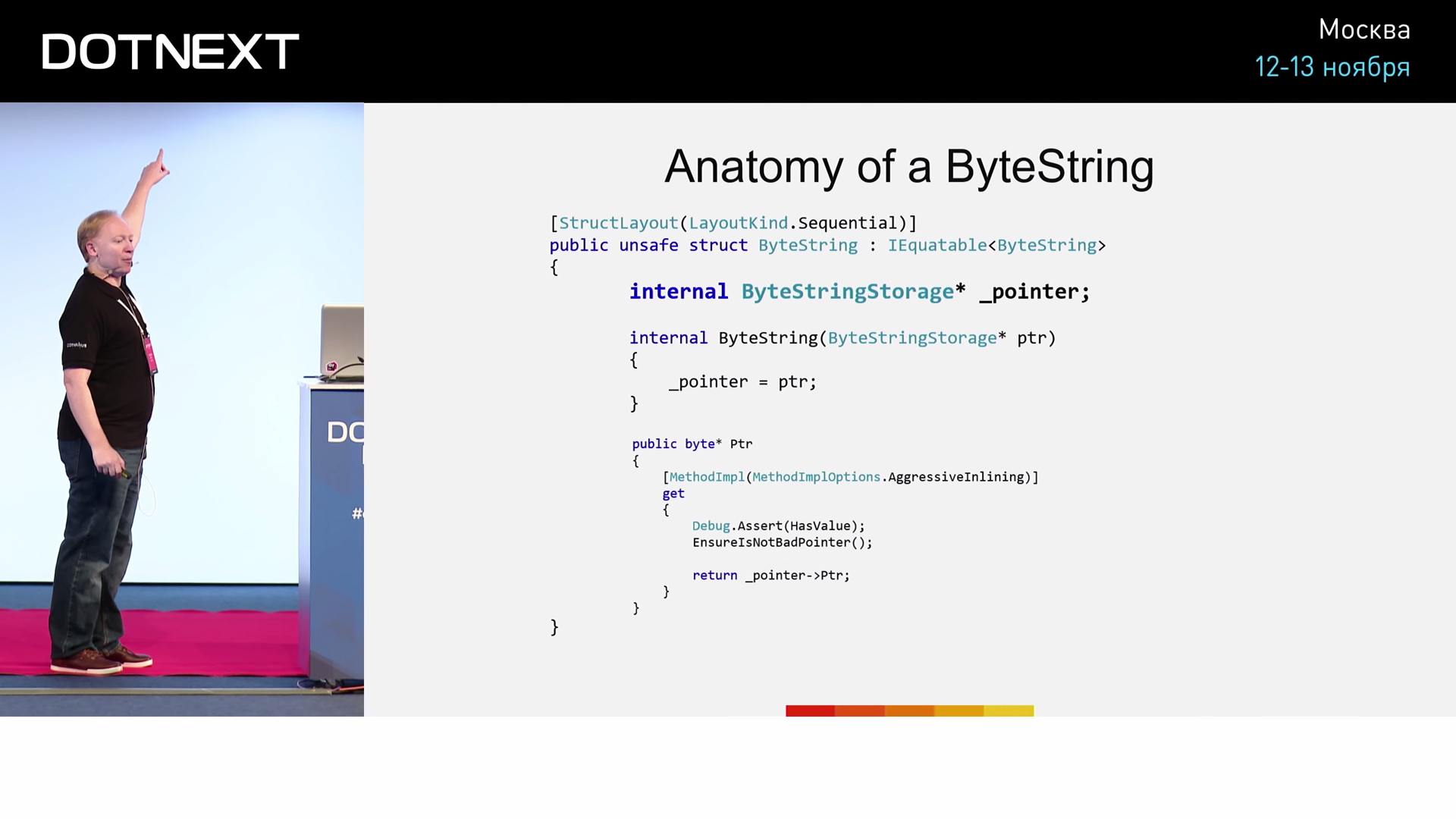
And now our ByteString is 8 bytes. Cool after all! But I want to ask the question: and yet, how much does it cost us to actually transfer ByteString as a parameter? The best way to find out is to conduct an experiment. Experimenting performance specialist forced constantly.

Let ByteString "a" specified inside the UsingByteString method. We will not perform any operations, the method should simply return "" . The compiler needs to specify that the method is “cold”. The “hot” method will always work faster - the purity of the experiment will be broken, the performance indicator will be distorted for the better. I will remind that ByteString , according to our implementation, should occupy 8 bytes. Below, we implement the UsingLong method, which performs the same actions (returning a value) on an 8-byte long variable. If ByteString a ByteString through a pointer is no more complicated than controlling a variable of type long, then UsingByteString and UsingLong work in equal time. As the implementation of ByteString we take the following:
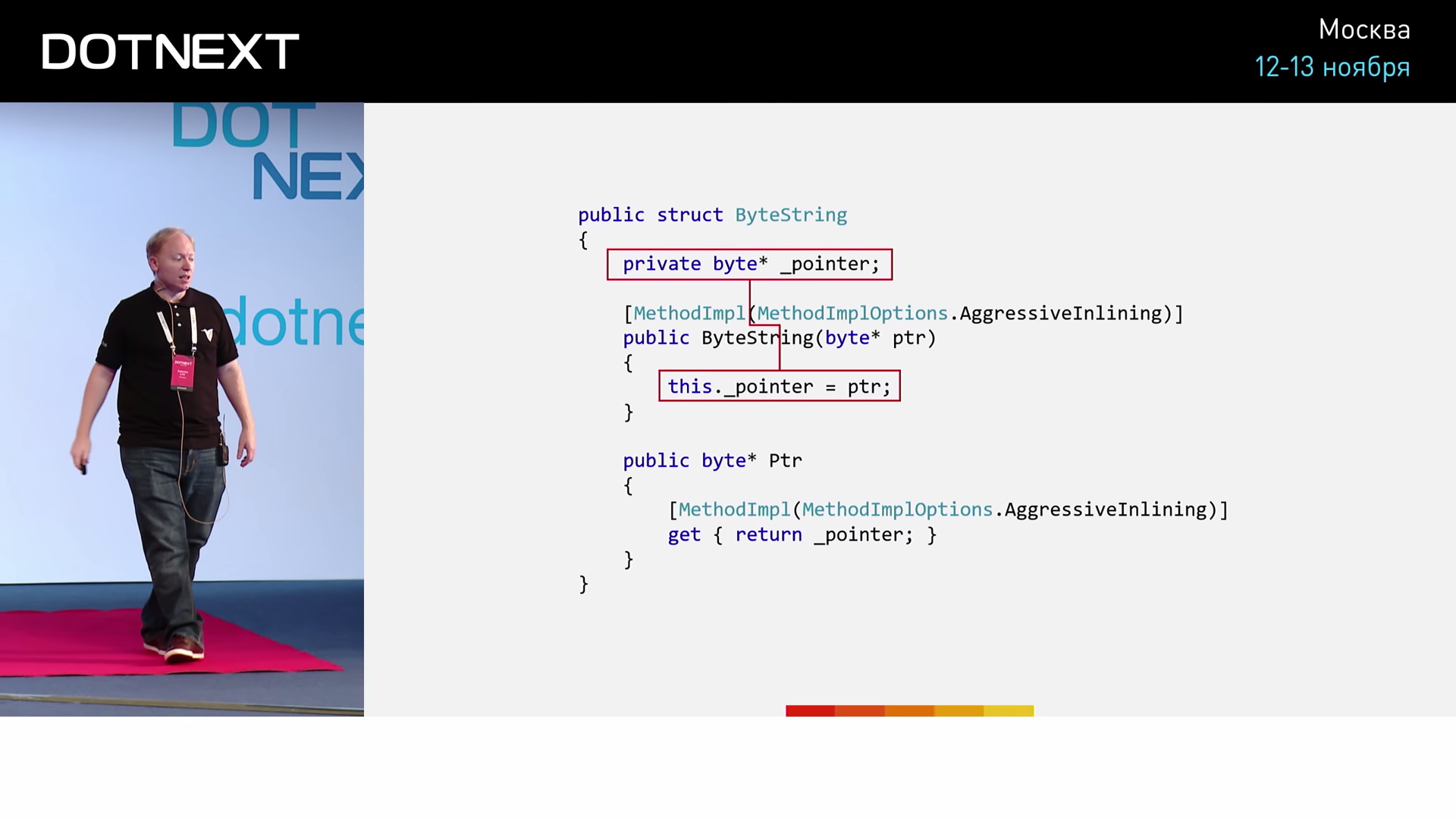
The implementation is simplified to a minimum, but it is quite suitable for our experiment. Creating an instance of the structure, we assign the value to the pointer. So, first we test on the variable long . The starting point of our program:

The value of the long variable is obtained from the static global variable. Then run our method, and save the returned value to the variable "a" . And, to prevent the compiler from intervening and optimizing anything here (and he does it only when all the actions of the code are strictly deterministic, in particular, there are no side effects), add an operation with a side effect - execute output "a" in console. Run the program and get the following result:
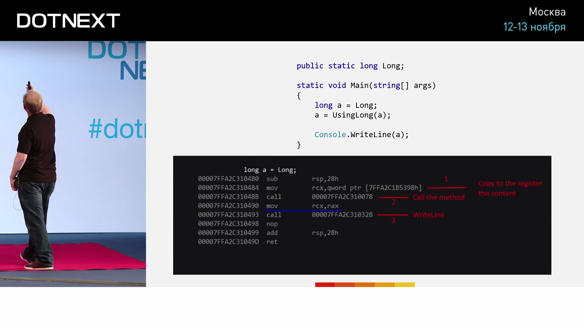
So, the first mov operation moves the first parameter of the method to the register RCX . Next comes the call operation — a function call, after which the value is copied from the RAX register to the RCX register — the value written by the function is returned to the variable "a" . The next call is a call to the WriteLine method. Now repeat the same thing, but with a ByteString . Code to run:

We declare a static global pointer variable. The Main code is similar: we initialize the new ByteString , call the UsingByteString method, UsingByteString returned value to the variable "a" and output its value to the console; in order to avoid any problems with Console.WriteLine , we add here an explicit cast to the long type. The results of the program:

In the same way, saving to the RCX register is performed, the method is RAX in the same way, the resulting value is copied from the RAX register to the RCX register in the same way, and the call to WriteLine occurs in the same way. The results are the same!
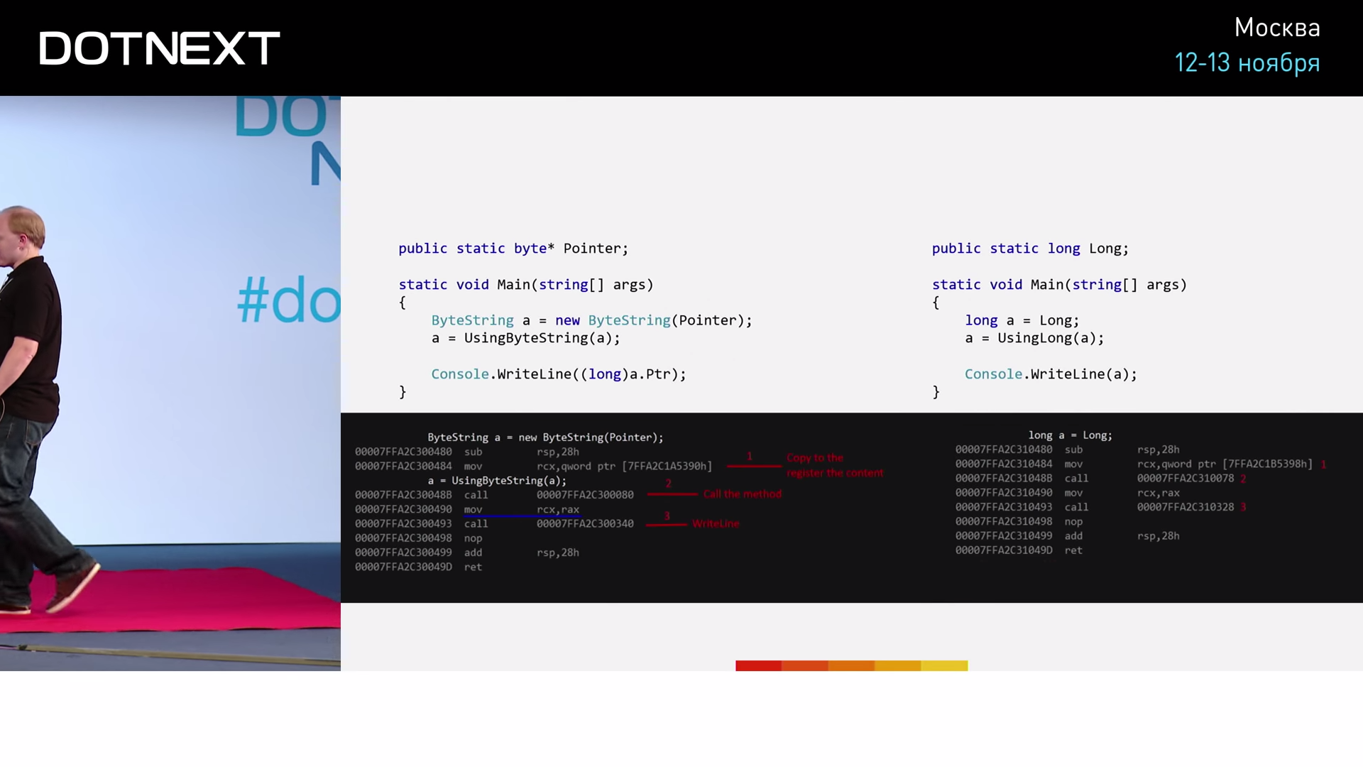
It turns out that, despite the obvious semantic difference, at the level of the JIT compiler, these two pieces of code are worked out identically. Perhaps you guess something. But be patient, the second part of the story is ahead.
Branch elimination
On the sly, the JIT compiler optimized something from us. We illustrate with another example:
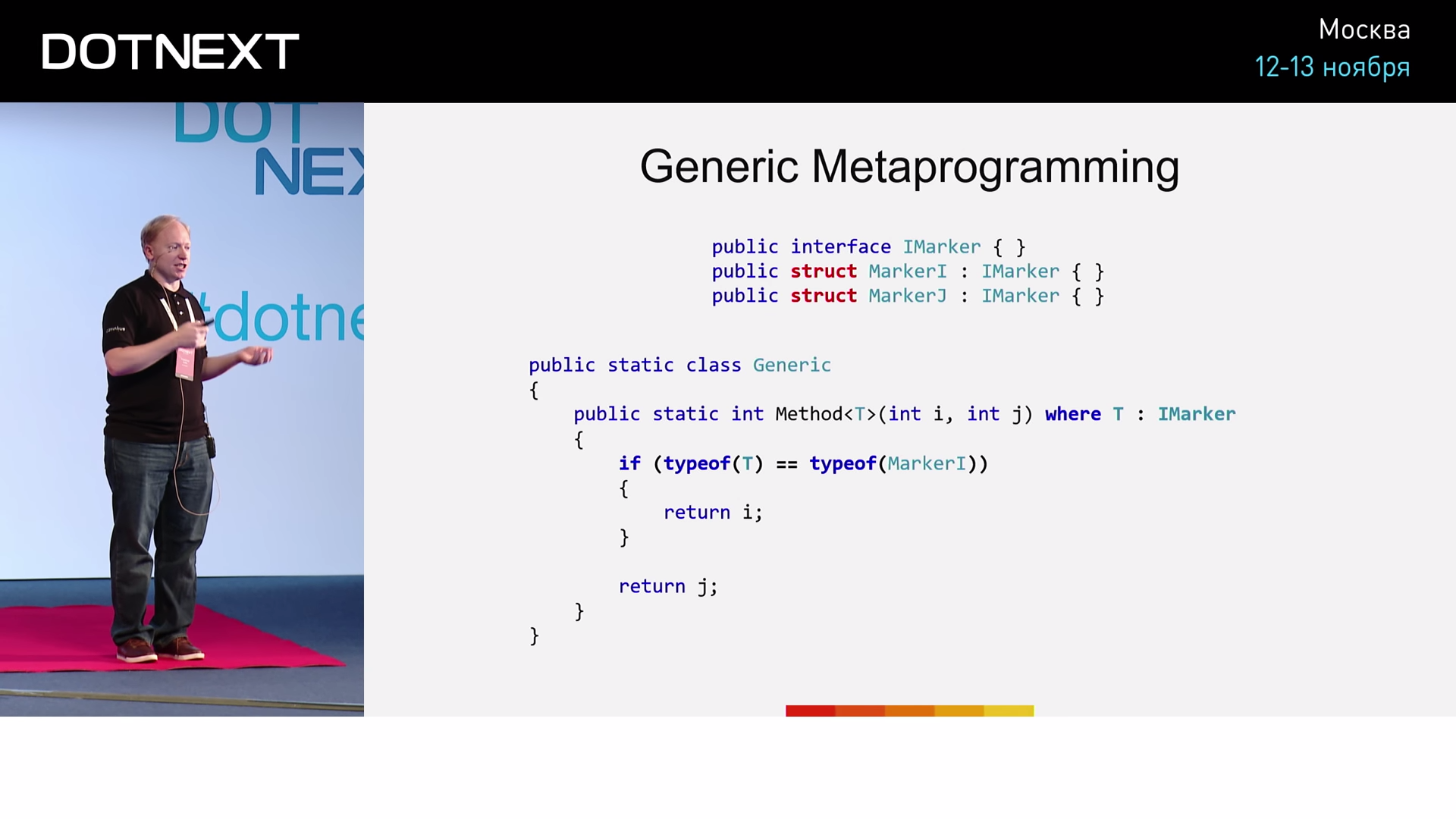
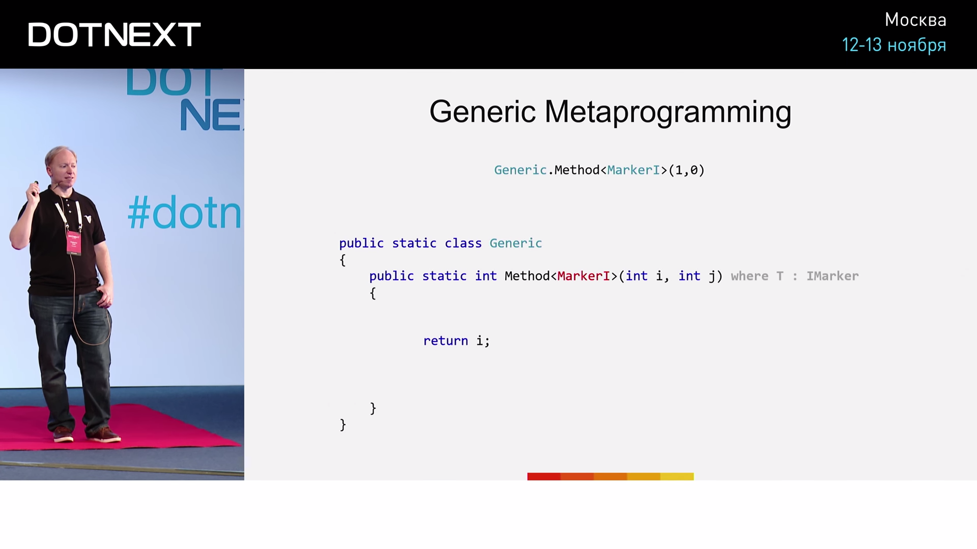
Suppose we have an empty IMarker interface and its two implementations, MarkerI and MarkerJ . However, importantly, we declare MarkerI and MarkerJ structures, not classes, as usual. Below we define the Method method, for which: - a type parameter belonging to the IMarker interface; i and j are input parameters of type int . Inside the method, we perform a simple operation: if T is equal to MarkerI , then we will return the value of i ; if T is equal to MarkerJ - we return j . Run the method with the MarkerI parameter.
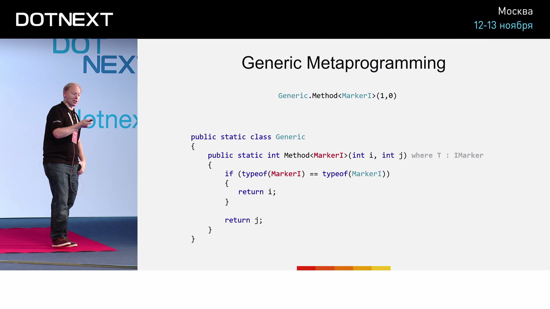
How exactly will the JIT compiler handle such a call? He will see the Method method and the MarkerI parameter that is passed to him. He then performs a check on the identity of MarkerI to the MarkerI interface, and, considering that the condition is fulfilled, will proceed to the execution of the method body. And further, analyzing the condition of the if statement, the compiler will perform a rather interesting operation: it will check whether MarkerI type is equal to MarkerI type and, of course, will be true . However, since MarkerI is a structure, not a class, the compiler considers that true in this case is constant and decides to remove the if statement from the code (along with what follows after it), leaving only the body commands if. The code will look like this:
Now run the method with the MarkerJ parameter.

This time, the analysis of the condition of the if statement will give a value of false (the transferred type MarkerJ not equal to the type MarkerI ). In the same way, the compiler will consider that in this case false is a constant, which means you can remove the if construct as a whole along with its contents. Thus, we observed the generation of code for two different branches by the JIT compiler.
Why do we need generic metaprogramming?
For C ++ programmers, I’ll say: for the same reasons as you. For everyone else, it allows you to:
- avoid frequent virtual calls;
- adapt the algorithms taking into account how we plan to use them (for example, how often);
- use the capabilities of the JIT compiler (definition of the values of constants and simple expressions) - get improved, “compacted” code;
- avoid invariant conditions (we cannot predict a branch of execution, but we can minimize the number of branches).
For a more visual presentation, I will give you an example of applying generalized metaprogramming. Let's talk about object pools.
Object Pools
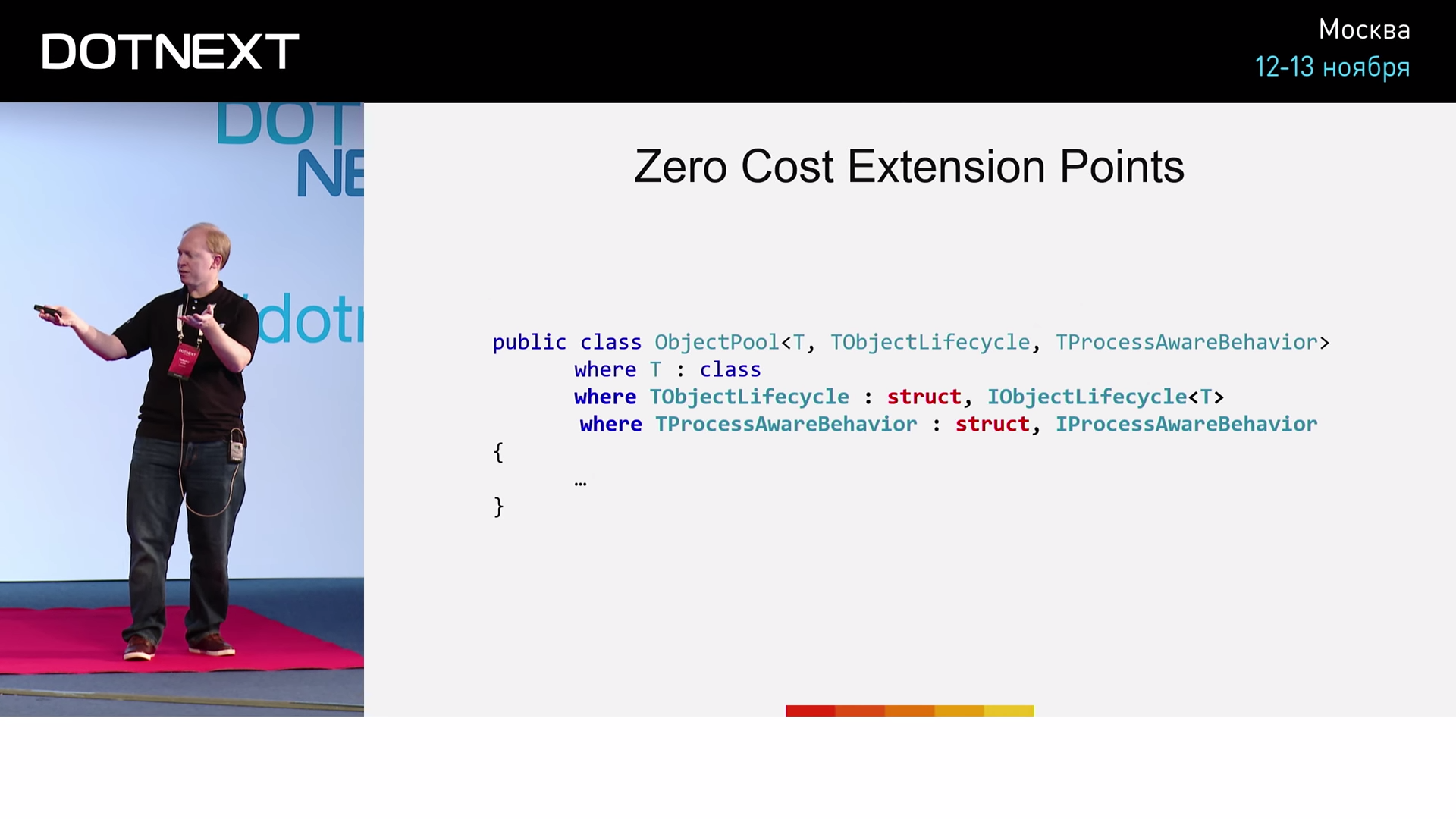
In essence, we have some type and we have a set of objects of this type - we get a pool. But the object after all has a life cycle: once it is created, and sooner or later we will need to remove it from memory (having contacted uncontrollable memory, we are forced to do removal literally with our hands). There is another nuance. Perhaps we want to make the object specially sharpened for a particular processor. If the last time some object was received by us from processor No. 1, then we would like further work with this object to occur as soon as possible and on the same processor No. 1. A typical implementation of the allocator today looks like this:
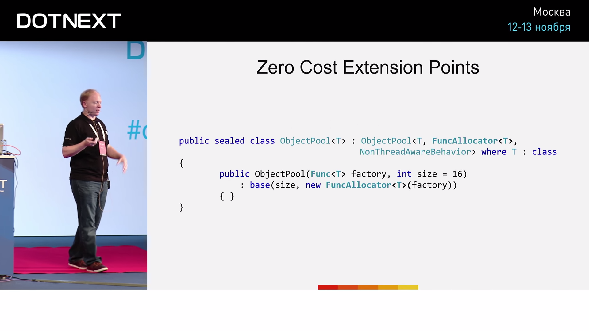
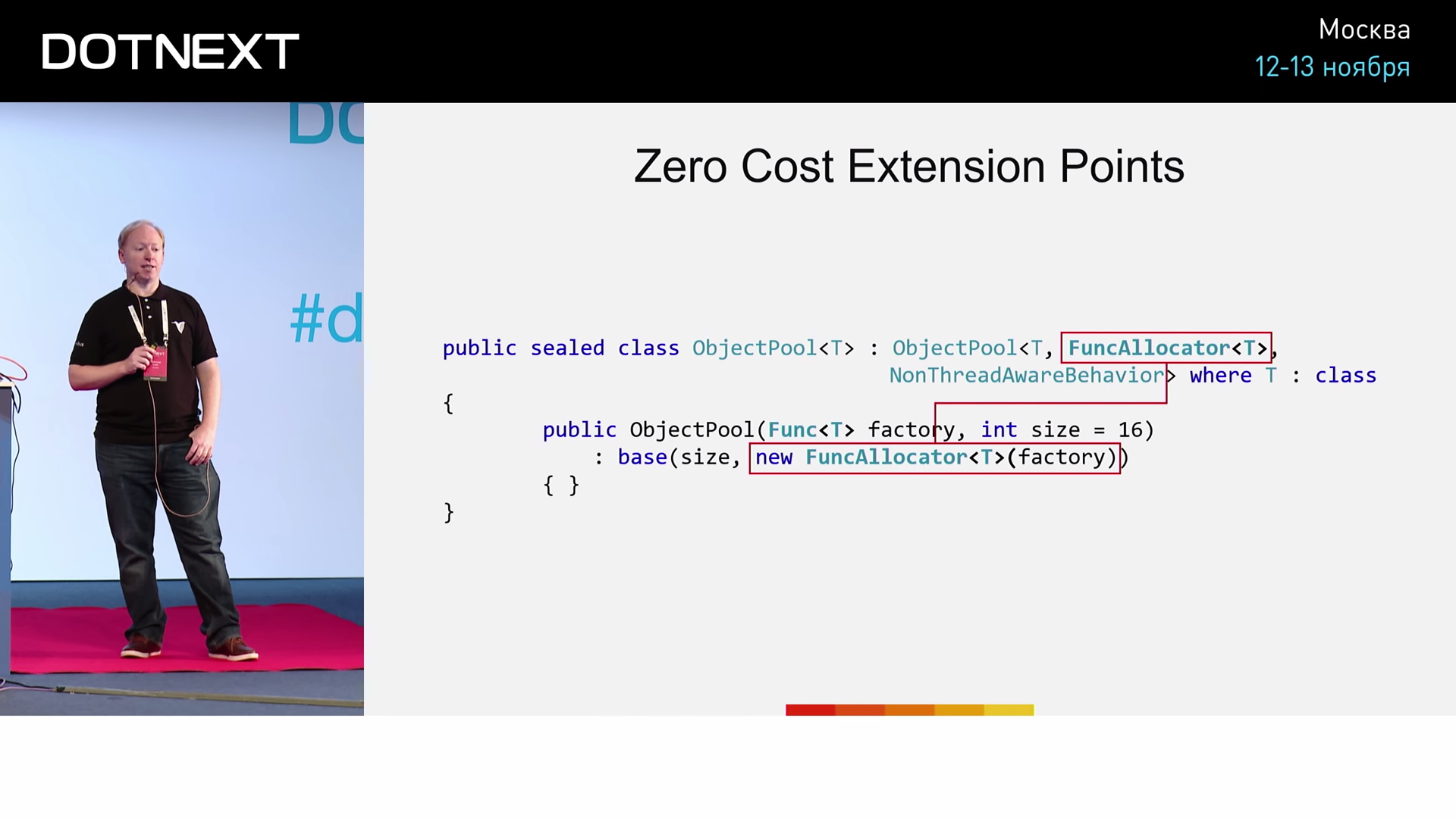
We have an object pool with NonThreadAwareBehavior. At the input to the constructor, we pass the function factory, which is able to create the object we need. The trick is that we will adjust the data types.
Compare two implementations:
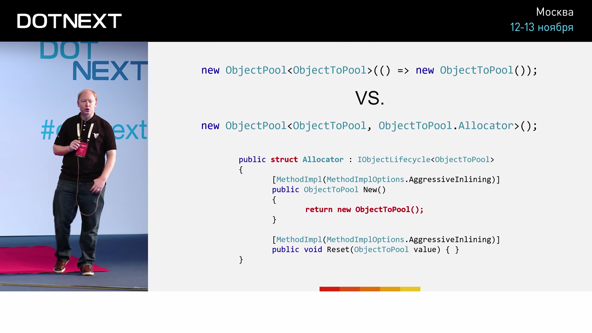
The first uses the classic approach just introduced. In the second, an explicit allocator is used, represented by an ordinary structure. To create a new pool object, in this case, we just need to use the New operator. Now we will test and compare these two implementations.
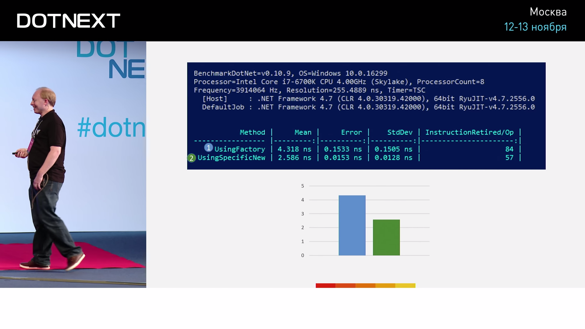
We can see that the implementation with the factory involved 84 assembler commands, and the implementation with New only 57. That is, the variant using New turns out to be more efficient by 1.7 times. How important is this distinction to us? Let's try something more interesting - let's implement an associative array (Dictionary).
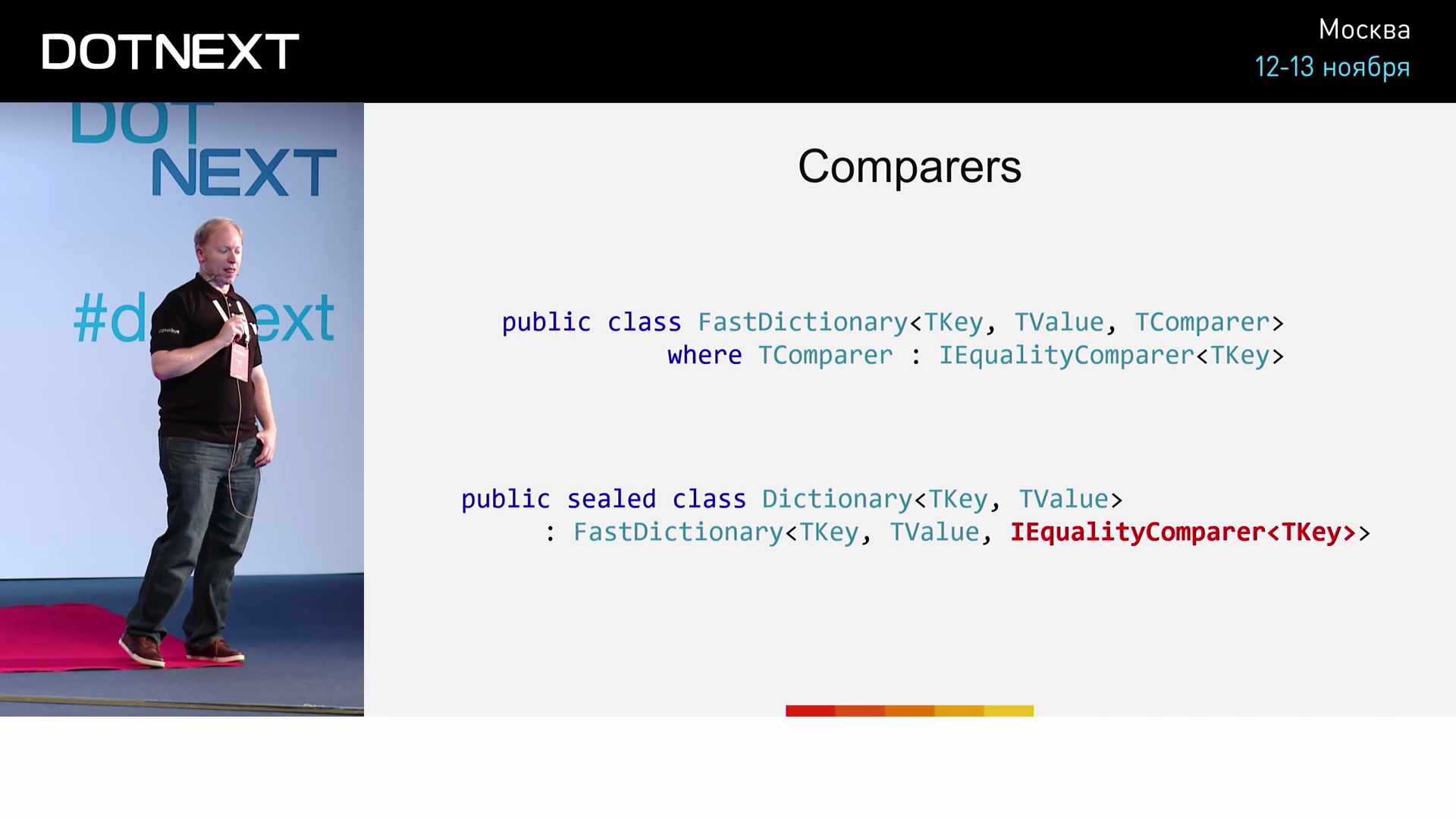
In addition to the usual two key and value arguments, let's declare the third one - a comparator. A classic implementation that matches our wishes will look something like this:

We specify the IEqualityComparer interface as a comparator. The implementation of NumericEqualityComparer quite simple:
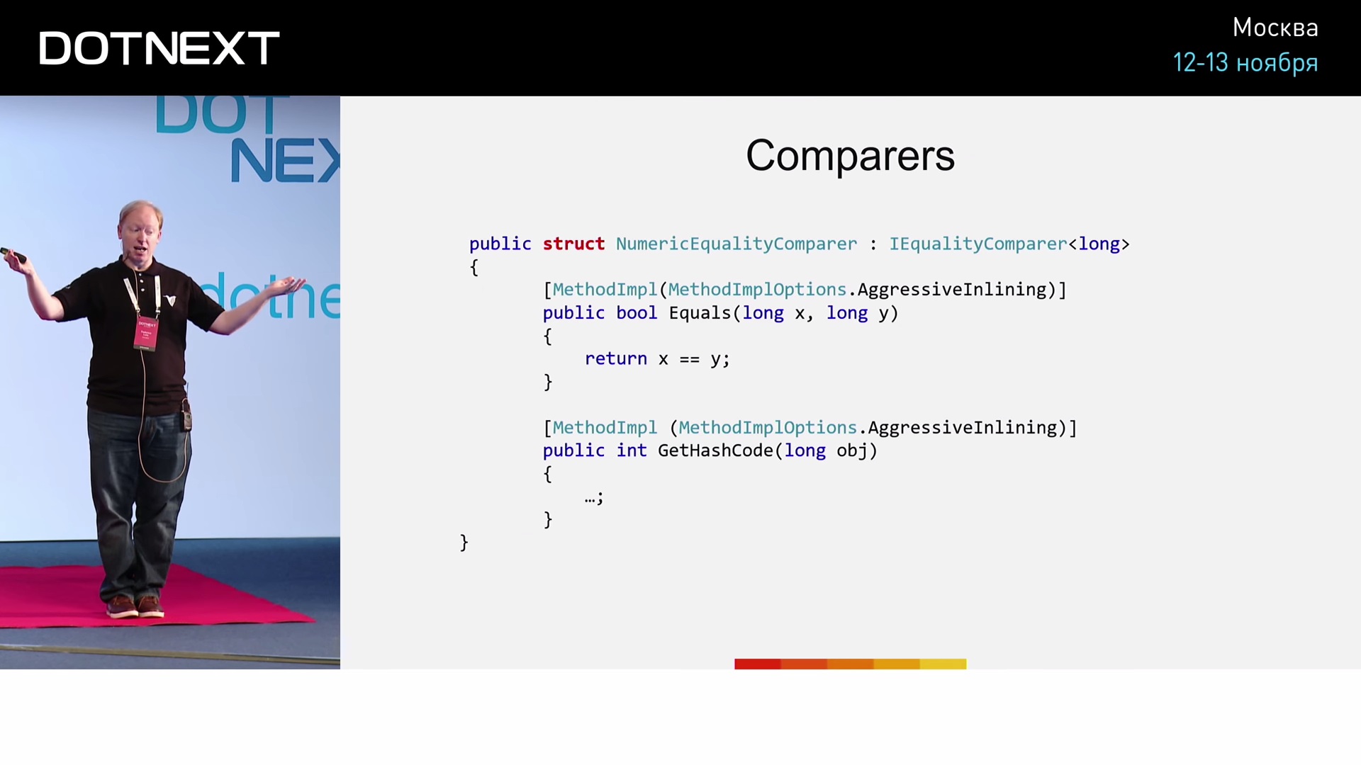
In this case, the NumericEqualityComparer is a structure that implements the IEqualityComparer interface for the long type. The Equals method simply returns the result of checking for the equality of the two long values passed to it. Pay attention to a special instruction for the implementation of the method - AgressiveInlining , upon seeing which, the JIT compiler will, if possible, execute the method as embedded. We will test three different implementations:
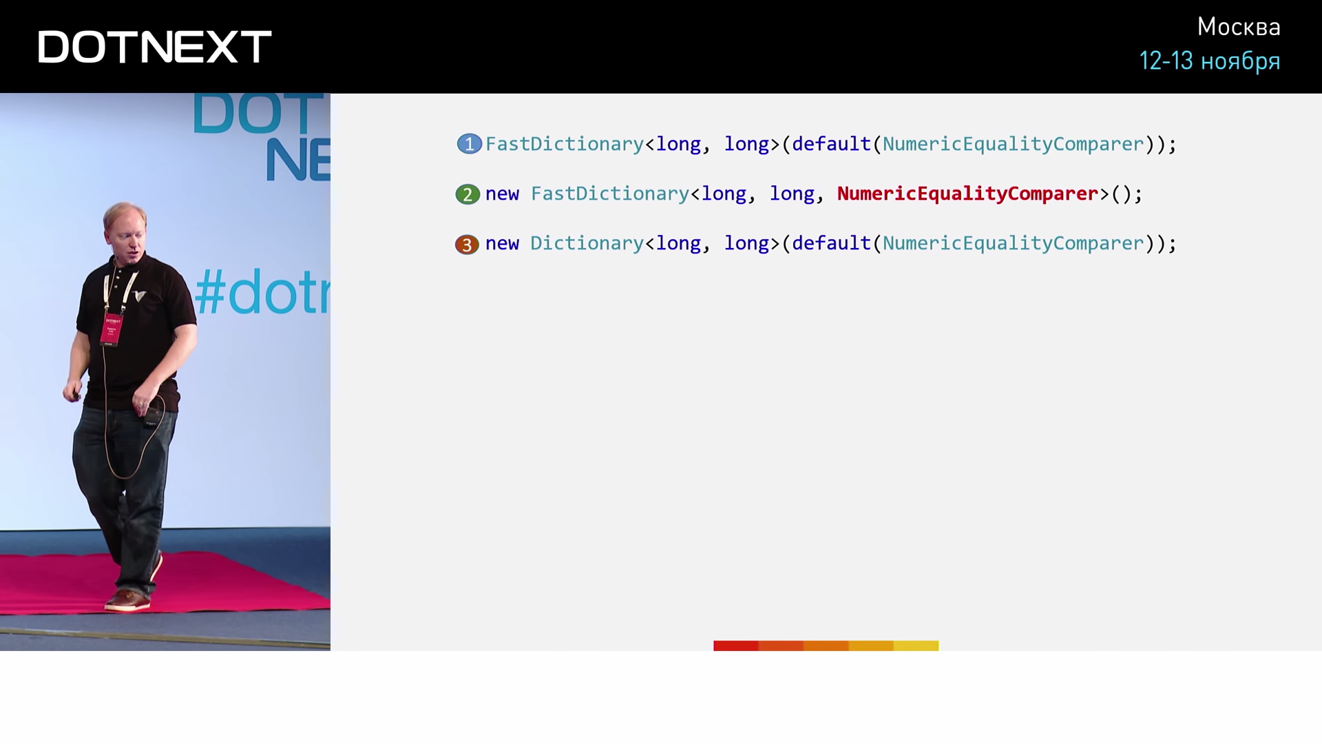
In the first case, we implement typical for .NET using an associative array using the interface. In the second case, bypassing the use of the interface, we try to pass our NumericEqualityComparer directly as a type. The third option we need to complete the picture. Here we do the same thing using the CoreCLR associative array. Test results give:
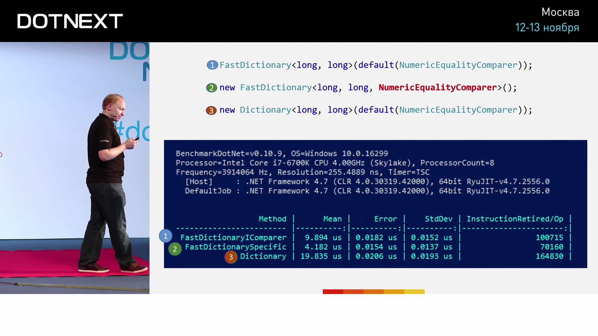

Obviously, FastDictionary algorithms are faster. But besides, we see that direct use of the NumericEqualityComparer type is NumericEqualityComparer efficient than using the interface more than twice. I have presented you with a few examples. Is it objective to use them as benchmarks? The answer is no. We need to conduct a real test.
From here we see that in fact the comparators were not built in: they turned out to be too large. And yet, the use of FastDictionary already increases our productivity by 3.25 times. Not any use of FastDictionary will give us a similar result, so it is important to understand what caused it in this particular case. The optimizations performed by JIT compilers are far from as simple as they seem.
Constants
One more example:

The doDispose flag is assigned a calculated value. JIT- , (, , , , ). , , . . , , , . :
( : TEvictionStrategy TEviction )
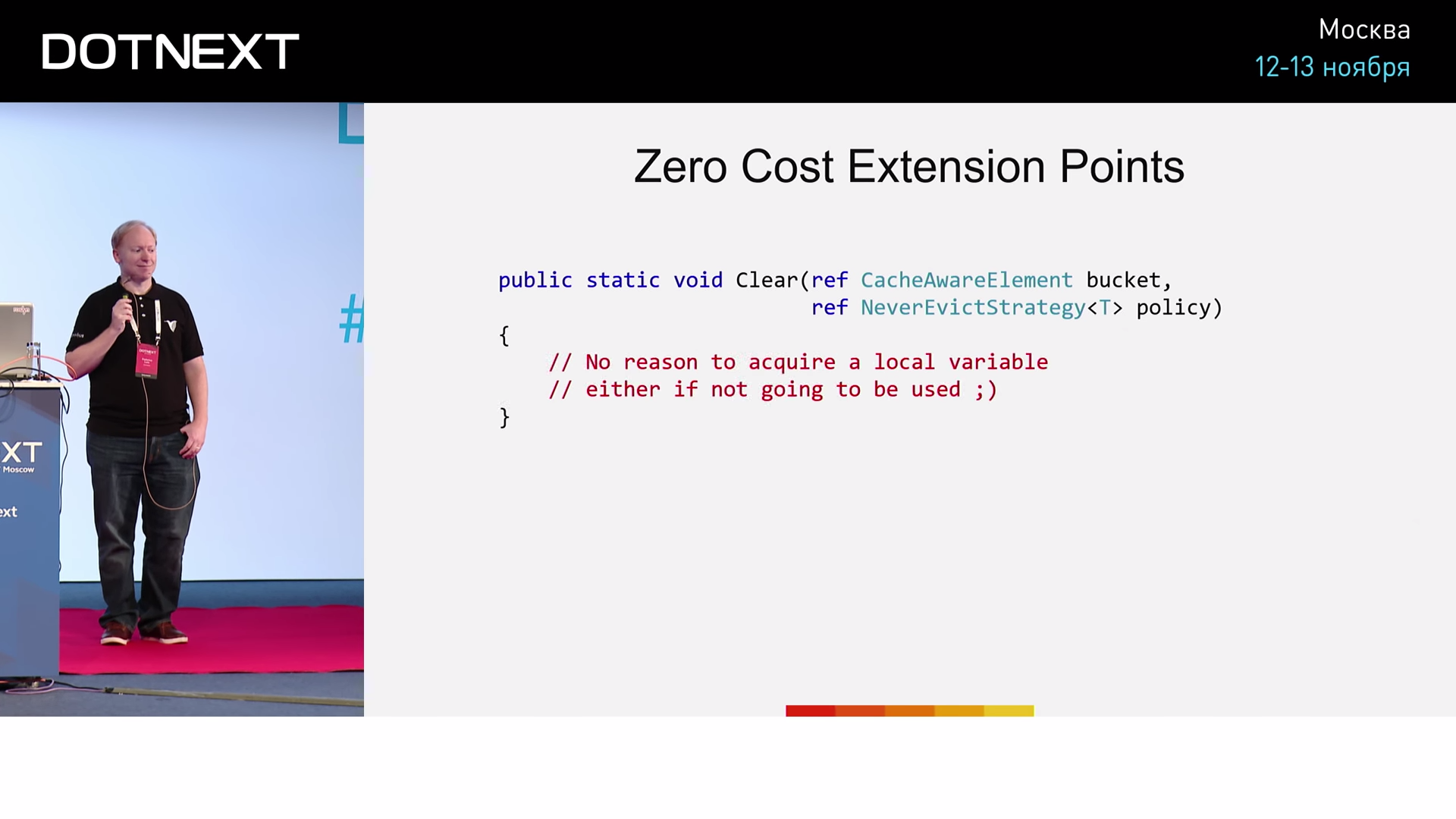
Clear , . , ? : (, 15 ). .

IEviction — . AlwaysEvictStrategy NeverEvictStrategy , : « » « ». , AlwaysEvictStrategy , NeverEvictStrategy CanEvict , true false . Clear :
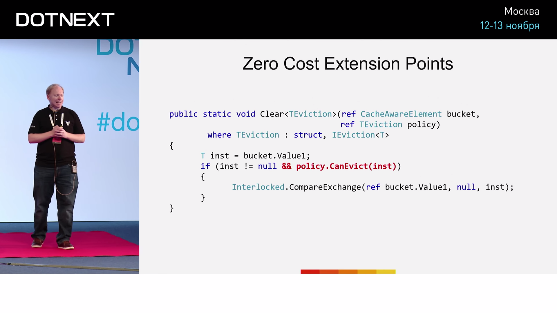
bucket . , CanEvict , , . . ( ), . AlwaysEvictStrategy , :
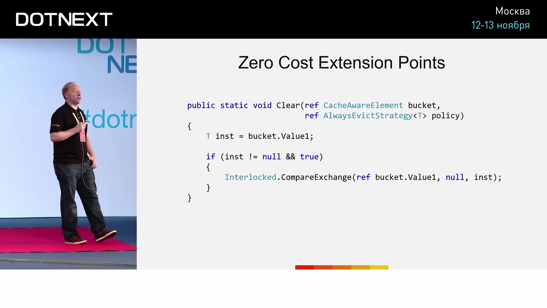
, , AlwaysEvictStrategy .

CanEvict true . if :
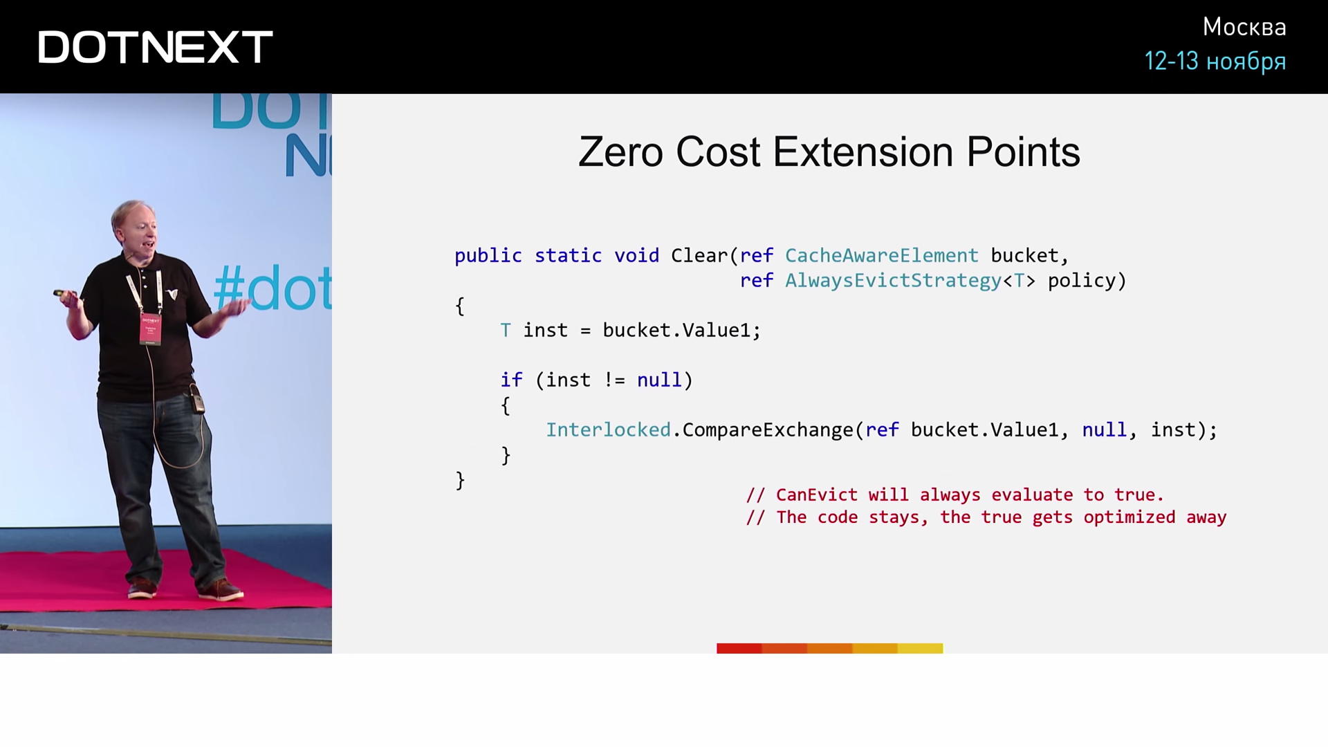
, NeverEvictStrategy , :
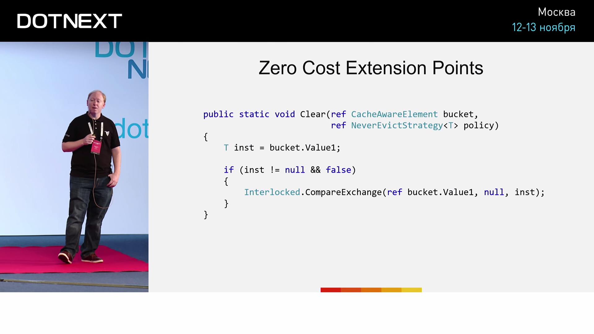
if false , CanEvict .

, , , if- :

inst ? :
?

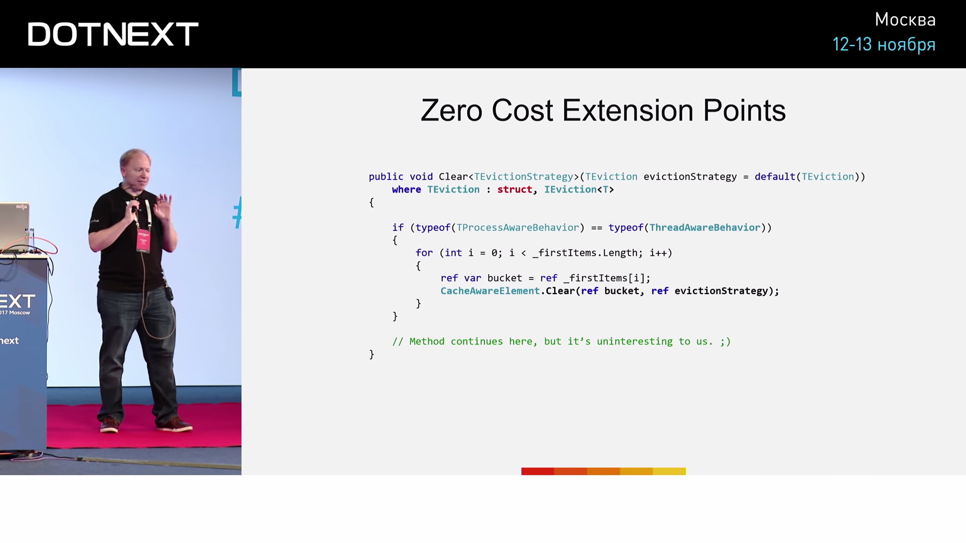
Clear . :

for, .
Zero Cost Façade
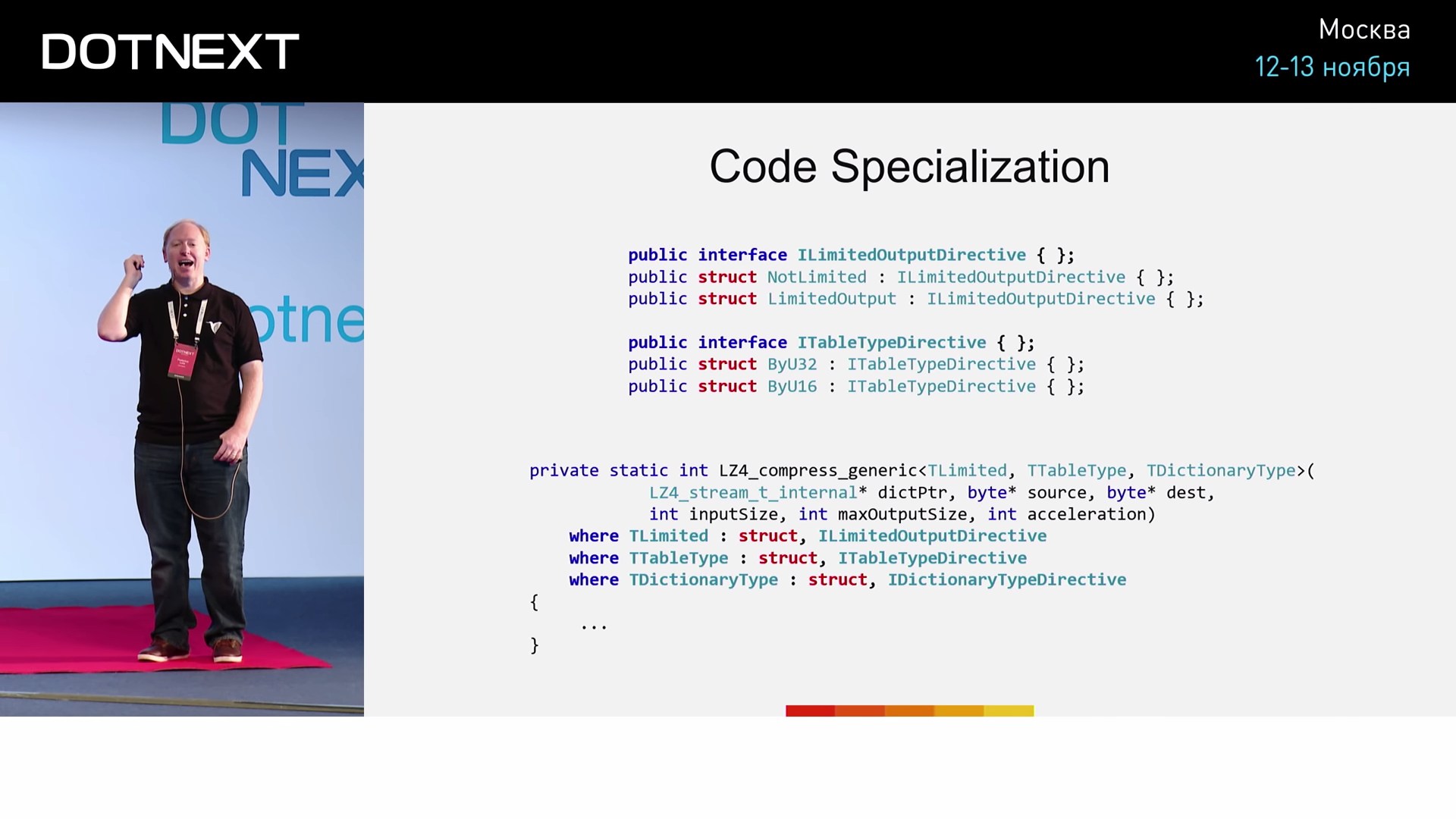
. , ILimitedOutputDirective , NotLimited LimitedOutput . ITableTypeDirective ByU32 ByU16 .

:
:
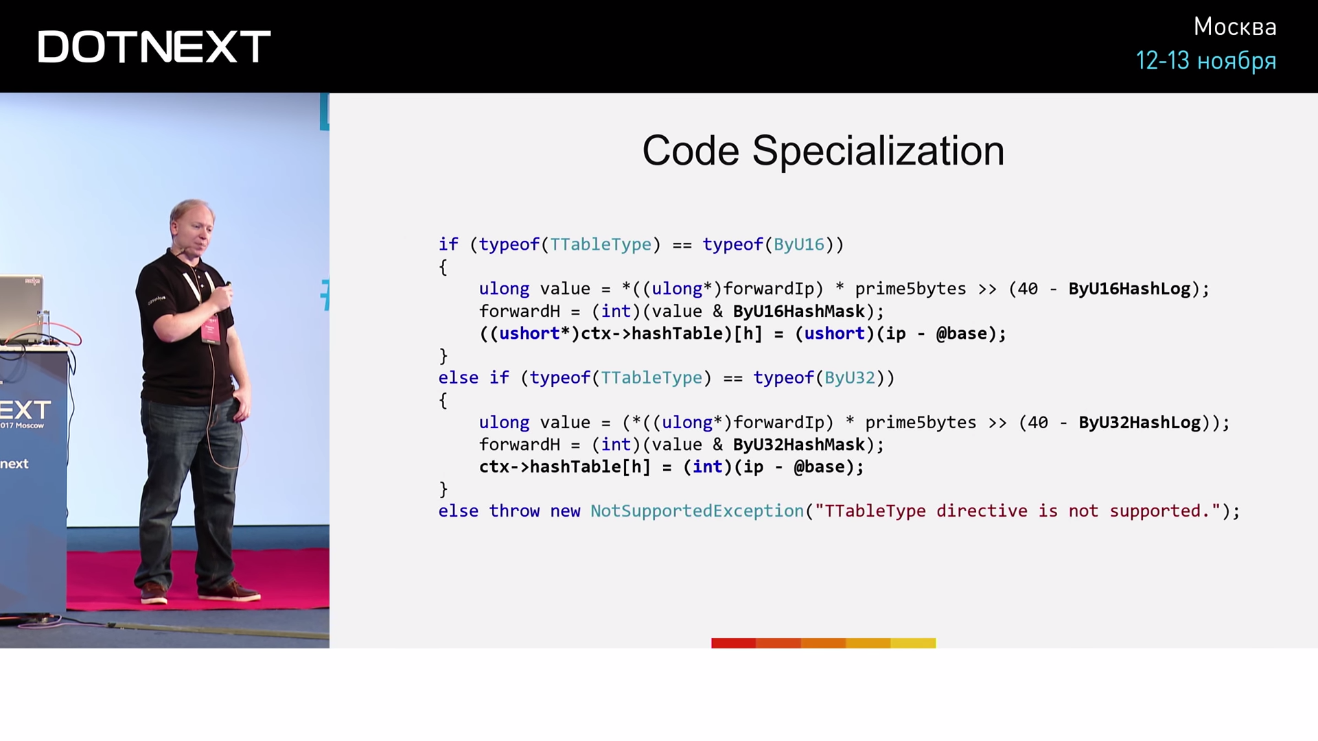
ByU16 , if. ByU32 — if. ByU32 , ByU16 , . . , «Zero Cost Façade». .

IUnmanagedWriteBuffer : UnmanagedStreamBuffer ( , , , , ) UnmanagedWriteBuffer ( ). , . .

, , BlittableWriter — , TWriter . , , :

WriteNumber , . AgressiveInlining . , , — . JIT- , , . ? , , .
, , : .
?
6 JSON-, - . 500 ( 8 ). , 3 . 2 , 2- . , , 6,6 . , , , , Raspberry Pi. . , , 1000 . , — .
Summarizing
? -, , . , .
, :
- ;
- :
- ;
- ;
- !
- ( Rust, « » — , );
- ( C# shapes and extensions );
- ( ).
C#- . , -, «shapes & extensions». , , C#.
- C :
- ;
- :
- ;
- ;
- ;
- .
. , . , , , ( Corvalius).
: , , . . 6 64 , 17% . , , — . ? I/O, , , . ! , .
What's next?
, !
- RavenDB 4.0: , Federico Lois ;
- Local (arena) Memory Allocators — John Lakos [ACCU 2017] ;
- Carl Cook «When a Microsecond Is an Eternity: High Performance Trading Systems in C++» ;
- An Overview of Program Optimization Techniques — Mathias Gaunard [ACCU 2017] ;
- MIT 6.172 Performance Engineering of Software Systems, Fall 2010 — BTree Write Cliff ;
- Understanding Flash: The Write Cliff (SSD);
- Oren Eini — (Federico Lois );
- CoreCLR ;
- BenchmarkDotNet .
Minute advertising. As you probably know, we do conferences. The nearest .NET conference - DotNext 2018 Piter . It will be held April 22-23, 2018 in St. Petersburg. What reports are there - you can see in our archive on YouTube . At the conference, it will be possible to chat live with the speakers and the best experts on .NET in special discussion zones after each report. In short, come in, we are waiting for you.
')
Source: https://habr.com/ru/post/352362/
All Articles