What do we know about the terrain loss of machine learning?

TL; DR

1. In deep neural networks, saddle points are the main obstacle for learning, rather than local minima, as previously thought.
2. Most local minima of the objective function are concentrated in a relatively small subspace of the scales. Networks corresponding to these minima give approximately the same loss on a test dataset.
3. The complexity of the landscape increases with the approach to global minima. In almost the entire volume of the weights space, the overwhelming part of the saddle points has a large number of directions, from which one can escape. The closer to the center of the cluster minima, the smaller the “escape directions” of the saddle points encountered on the path.
4. It is still unclear how to find a global extremum in the subspace of minima (any of them). It seems that it is very difficult; and not the fact that a typical global minimum is much better than a typical local one, both in terms of loss and in terms of generalizing ability.
5. In clusters of minima, there are special curves connecting local minima. The loss function on these curves takes only slightly larger values ​​than in the extremes themselves.
6. Some researchers believe that wide minima (with a large radius of the “pit” around) are better than narrow ones. But there are quite a few scientists who believe that the connection between the width of the minimum and the generalizing ability of the network is very weak.
7. Skip connections make the terrain more friendly for gradient descents. It seems that there is no reason not to use residual learning.
8. The wider the layers in the network and the smaller (to a certain limit), the smoother the landscape of the objective function. Alas, the more redundant the network parametrization, the more neural network is subject to retraining. If ultra-wide layers are used, then it is easy to find a global minimum in the training data set, but this network will not be generalized.

Everything, scroll further. I even will not put KDPV.

The article consists of three parts: a review of theoretical papers, a review of scientific works with experiments, and a cross-comparison. The first part is a bit dry, if you get bored, skip right to the third.

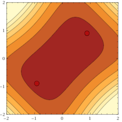
But first, a clarification on point two. The claimed subspace is small in total volume, but can be arbitrarily large in scope when projected onto any straight line in hyperspace. It contains both clots of minima, and simply areas where the loss function is small. Imagine two consecutive linear neurons. At the exit from the network will be the value $$$w_1 w_2 x$ . Suppose we want to want to teach them to play the identity function $$$y (x) = x$ . If we apply to the L2 loss network, then the surface of the error function will look like $$$E (\ theta) = (w_1 w_2 x - x) ^ 2 = x ^ 2 (w_1 w_2 - 1)$ :

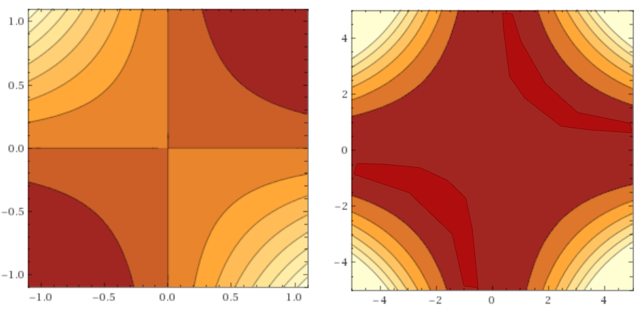
Where the abscissa is postponed $$$w_1$ , and on the ordinate - $$$w_2$ .

It's obvious that $$$w_1 = 1, w_2 = 1$ ideally reproduce identity-function, but do the same $$$w_1 = -1, w_2 = -1$ and for example $$$w_1 = -5, w_2 = - \ frac {1} {5}$ . All these are global minima (their infinite number), and the red-burgundy area on the graphs is a subspace of minima (as you see, it extends infinitely along both axes, but becomes increasingly thinner as it moves away from zero). We observe this behavior due to the symmetry of the weights, and this phenomenon is characteristic not only of linear networks. It is partially treated by regularization, but even so there are two global minimums. $$$w_1 = 1, w_2 = 1$ and $$$w_1 = -1, w_2 = -1$ (plus or minus distortion from regularization).

')
In the future, under the "global minimum" I will understand "any of the identical global minima", and under the "clot of minima" - "any of the symmetric clots of local minima".

Review of theoretical works

As is known, neural network training is the search for a minimum of the target loss function. $$$E (\ theta)$ in the space of scales $$$\ theta$ . Alas, finding the global minimum of an arbitrary differentiable function belongs to the class of NP-complex problems [1]. In addition, neural networks can have very different architectures and accept any data as input, so there is no hope for a deep analysis of a single formula with clearly defined restrictions. Function $$$E (\ theta)$ incredibly multidimensional, hence the brute force method is also non-trivial to apply here. However, even some general facts about the typical landscape $$$E (\ theta)$ can bring considerable benefits: at a minimum, set the general direction of practical research.

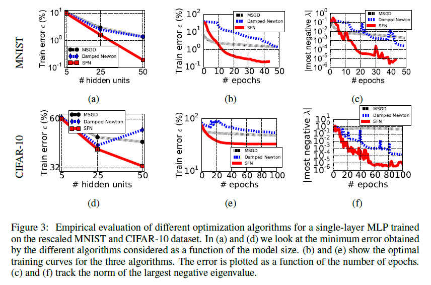
Until recently, there were few people willing to tackle such a titanic task, but at the beginning of 2014, the article by Andrew Saxe and others [2] was published, which discusses the non-linear learning dynamics of linear neural networks (the formula for the optimal learning rate is given) and the best way to initialize them (orthogonal matrices). The authors get interesting calculations based on the decomposition of the weights of a network in SVD and theorize how the results can be transferred to nonlinear networks. Although the work of Saxe is not directly related to the topic of this article, it prompted other researchers to take a closer look at the dynamics of learning neural networks. In particular, a little later in 2014, Yann Dauphin and the team [3] review the existing literature on learning dynamics and pay attention not only to the Saxe article, but also to the work of Bray and Dean [4] from 2007 about statistics of critical points in random Gaussian fields. They propose a modification of the Newton method (Saddle Free Newton, SFN), which not only better escapes from the saddle points, but also does not require the calculation of the total Gaussian (minimization follows vectors of the so-called Krylov subspace). The article demonstrates very nice graphics improving the accuracy of the network, which means SFN is doing something right. The Dauphin article, in turn, gives impetus to new studies of the distribution of critical points in the space of weights.



So, there are several areas of analysis of the stated problem.

The first is to steal from someone a little run-in mathematics and attach it to your own model. This approach was used with incredible success by Anna Chromanska and the team [5] [6], using the equations of the theory of spin glasses. They limited themselves to considering neural networks with the following characteristics:

• Direct distribution networks.
• Deep nets. The more weights, the better the asymptotic approximations work.
• ReLU activation features.
• L2 or Hinge loss function.

After which they imposed several more or less realistic restrictions on the model:

1. The probability of a neuron to be active is described by the Bernoulli distribution.
2. The activation paths (which neuron activates which one) are evenly distributed.
3. The number of scales is redundant to form a distribution function. $$$X$ . There are no scales whose removal blocks learning or prediction.
4. Spherical weight limits: $$$\ exists C: \ frac {1} {\ Lambda} \ sum_ {i = 1} ^ {\ Lambda} w_i ^ 2 = C$ (Where $$$\ Lambda$ - the number of scales in the network)
5. All input variables have a normal distribution with the same variance.

And a bit unrealistic:

1. Activation paths in the neural network do not depend on the specific $$$X$ .
2. Input variables are independent of each other.

On the basis of what received the following statements:

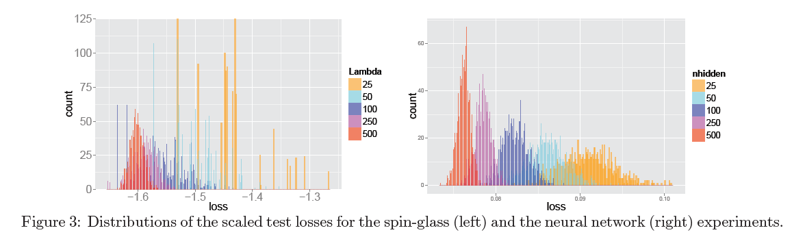
• The minima of the loss function in a neural network form a cluster in a relatively small subspace of weights. Beyond a certain limit, the values ​​of the loss function begin to exponentially decrease.
• For properly trained deep neural networks, most local minima are about the same in terms of performance on the test sample.
• The probability of being in a “bad” local minimum is noticeable when working with small networks and exponentially decreases with an increase in the number of parameters in the network.
• Let be $$$k$ - the number of negative eigenvalues ​​of the Hessian at the saddle point. The bigger it is, the more ways along which the gradient descent can escape from the critical point. For each $$$k$ there is some measure of the value of the objective function $$$E = - \ Lambda E (\ theta) _k$ starting at which the density of saddle points with such $$$k$ begins to decrease exponentially. These numbers are strictly increasing. In Russian, this means that the loss function has a layered structure, and the closer we are to the global minimum, the more there will be nasty saddle points from which it is difficult to get out.

On the one hand, we almost got a lot of proven theorems “for free”, showing that under certain conditions neural networks behave according to spin glasses. If something is able to open the infamous "black box" of neural networks, it is matan from quantum physics. But there is an obvious drawback: very strong initial premises. Even 1 and 2 from the group of realistic ones seem doubtful to me, what can we say about the group of unrealistic ones. The most serious limitation in the model seems to me to be the uniform distribution of activation paths. What if some small group of activation paths is responsible for classifying 95% of dataset elements? It turns out that it forms a network in the network, which significantly reduces the effective $$$\ Lambda$ .

There is an additional trick: Chromanska assertions are difficult to be refined. It is not so difficult to construct an example of weights representing a “bad” local minimum [7], but this does not contradict the message of the article: their approval must be carried out for large networks. However, even the provided set of weights for a moderately deep feed-forward network that poorly classifies, say, MNIST is unlikely to be a strong proof, because the authors argue that the probability of meeting a “bad” local minimum tends to zero, and not that they are not there at all. Plus, “for properly trained deep neural networks” is a rather loose concept ...



The second approach involves building a model of the simplest possible neural networks and iteratively bringing it to a state where it can describe modern machine learning monsters. We have a basic model for a long time - these are linear neural networks (i.e., networks with the activation function $$$f (x) = x$ ) with one hidden layer. They are amenable to analysis, and they have long been engaged in, but the results of these theoretical studies were of little interest to anyone, since, in general, linear networks are not very useful.

At least, there were very few people interested until recently. Using rather weak restrictions on layer sizes and data properties, Kenji Kawaguchi [8] develops the results of work [9] from as much as 1989 and shows that in certain linear neural networks with L2-loss

1. Though $$$E (\ theta)$ non-convex and non-concave
2. All local minima are global (there may be more than one)
3. And all the other critical points are saddles.
4. If a $$$\ theta$ - the saddle point of the loss function and the rank of the matrix product of the network weights is equal to the rank of the narrowest layer in the neural network, then the Hessian in $$$E (\ theta)$ has at least one strictly negative eigenvalue.

If the rank of the product is less, then the Hessian matrix can have zero eigenvalues, which means that we cannot so easily understand whether we have fallen into a weak local minimum or a saddle point. Compare with features $$$f (x) = x ^ 3$ at zero and $$$f (x) = \ max (0, x ^ 3) + \ min (0, (x + 1) ^ 3)$ at $$$x = 0.5$ .

After that, Kawaguchi takes into consideration the network with ReLu-activation, slightly weakens the limitations of Choromanska [6], and proves the same statements for neural networks with ReLu-nonlinearities and L2-loss. (In the following paper [10], the same author gives a simpler proof). Hardt & Ma [11], inspired by the calculations [8] and the success of residual learning, prove even stronger assertions for linear networks with skip connections: under certain conditions there are not even “bad” critical points without negative eigenvalues ​​of the Hessian (see [ 12] for a theoretical justification of why “short circuits” in the network improve the landscape, and [13] for examples of graphs $$$E (\ theta)$ before and after adding skip connection)

The accumulated knowledge base summarizes the very recent work of Yun, Sra & Jadbabaie [14]. The authors strengthen the Kawaguchi theorems and, like Chromanska, divide the space of weights of a linear neural network into a subspace that contains only saddle points, and a subspace that contains only global minima (necessary and sufficient conditions are given). Moreover, scientists finally make a step in the direction of interest to us and prove similar statements for nonlinear neural networks. Let the latter be done with very strong prerequisites, but these are prerequisites different from the conditions of Chromanska.

Review of works with visualization

The third approach is to analyze the values ​​of the Hessian in the learning process. Mathematicians have long known second-order optimization techniques. Machine learning specialists periodically flirt with them (with methods, not with mathematicians ... albeit with mathematicians, too), but even truncated second-order descent algorithms have never been particularly popular. The main reason for this lies in the cost of calculating the data required for the descent, taking into account the second derivative. Honestly calculated Hessian takes a square of the number of memory weights: if there are a million parameters in a network, then in the matrix of second derivatives there will be $$$10 ^ 12$ . But you still want to somehow calculate the eigenvalues ​​of this matrix ...

For the same reason, there are few works that allow us to look at the dynamics of change in the Hessian in the learning process. More precisely, I found exactly one work by Yann LeCun and the company [34] dedicated to this, and even then they work with a relatively primitive network. Plus, there are a couple of relevant notes and graphs in [3] and [12].

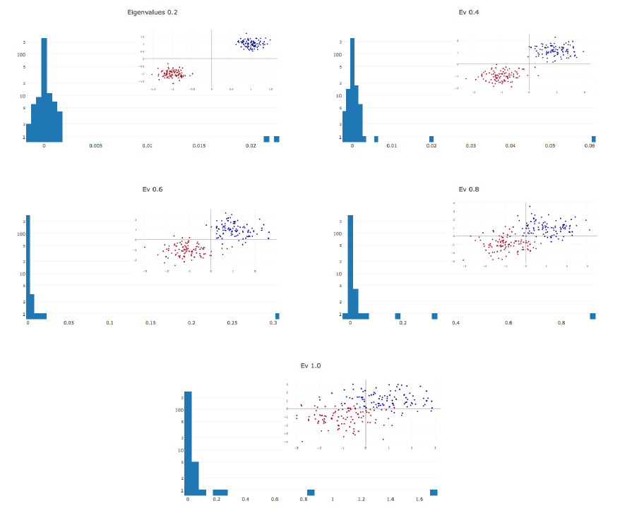
LeCun [34]: The Hessian consists almost entirely of zero values ​​throughout the course of training. During optimization, the Hessian histogram is further compressed to zero. Non-zero values ​​are unevenly distributed: a long tail is thrown in the positive direction, while negative values ​​are concentrated around zero. Often, it only seems to us that the learning has stopped, whereas we just ended up in a pool with small gradients. At the breakpoint, there are negative eigenvalues ​​of the Hessian.


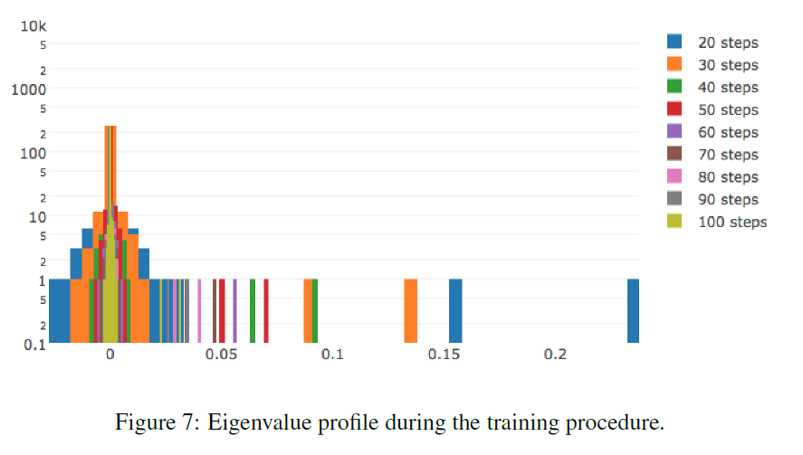
The more complex the data, the more elongated the positive tail of the distribution of eigenvalues.



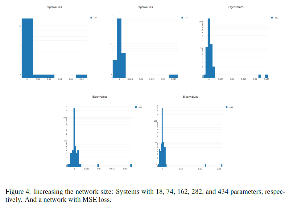
The more parameters in the network, the more stretched the histogram of eigenvalues ​​in both directions.



Dauphin et al. [3]: On graphs A and C along the axis $$$x$ the relative part of the negative values ​​at the critical point at which the learning stopped, according to $$$y$ postponed error on the training set. Graphs B and D show histograms of the eigenvalues ​​of the matrix of second derivatives for three points from graphs A and C, respectively. Please note that they are consistent with the LeCun histograms.

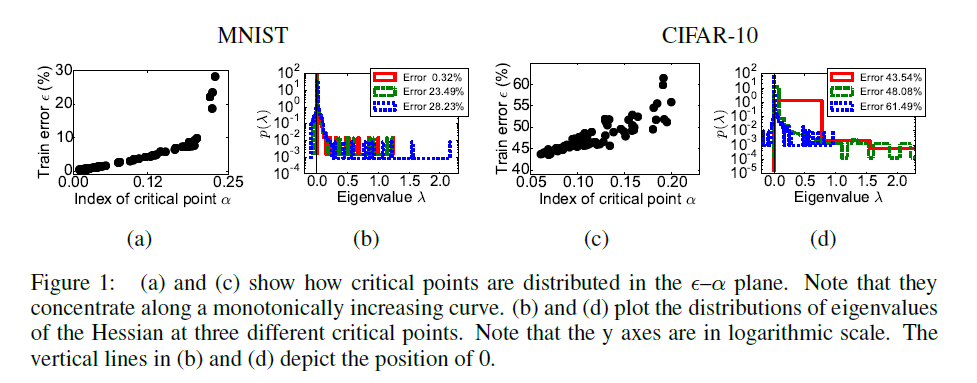
Clearly visible is the correlation between the number of directions of escape from the saddle point and the quality of the network in it.

Orhan & Pitkow [12]: The relative number of degenerate and negative negative Hessian values ​​are shown. The article says not exactly about the same thing as in [3] and [34], but on the whole the graphs indirectly confirm the results of the two previous works.



The fourth way - a direct analysis of the landscape $$$E (\ theta)$ by means of visualization of any projections. The idea is trivial, but, as already mentioned, it's not easy to apply it, because in $$$\ theta$ there may be millions of scales. Usually consider two types of visualization: the values ​​of the loss function when changing $$$\ theta$ in the space of weights along a curve and the graph of the loss function in the vicinity of a point at $$$\ theta \ in \ theta_0 + a \ vec {v_1} + b \ vec {v_2}$ where $$$\ vec {v_1}$ and $$$\ vec {v_2}$ - some vectors defining the plane of the cross section of the space of weights. In the case of a one-dimensional projection, it is common to visualize transitions from the initial state of the network to the final state (directly or along a learning curve) or between two final states; in the two-dimensional state, two most significant vectors are usually taken in the PCA decomposition of the final part of the learning curve. In addition to multidimensionality, the problem of visualization of the objective function is complicated by the fact that essentially the same minimums can have very different weights. For example, if the linear neural network weights in one layer decrease in $$$a$ once and in the next - in $$$a$ if we increase, then the resulting sets of weights and the area of ​​space around them will be very different, whereas the learned features will be essentially the same. Additional measurement for analysis - type of minimizer or parameters of a specific type of minimizer with which it was obtained $$$\ theta$ .

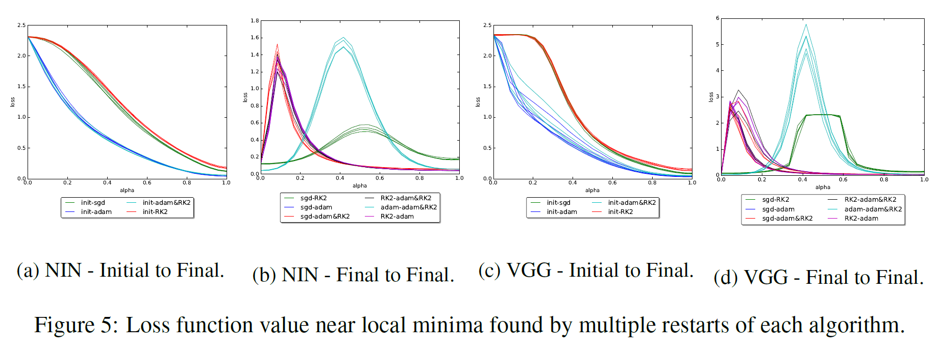
One of such works is [16]. In it, researchers look at the segment between the end points of launches with SGD, Adam, Adadelta and RMSProp. As in many other papers, it is found that different algorithms find characteristically different minima. Also, the authors of the article show that if during training you change the type of algorithm, then $$$\ theta$ will change course to another minimum. As a second bonus, researchers see how the landscape between the end points of batch normalization will affect the landscape, and conclude that, first, with batch normalization, the quality of the minimum obtained depends much less on the initialization point, and second, between the final $$$\ theta$ “walls” appear in the landscape of the objective function — narrow sections with a very large value. $$$E (\ theta)$ (it is not clear where it comes from and what to do with it). In any case, on the diagrams between the minima one can see the “hills” of loss, but not some complicated surface.



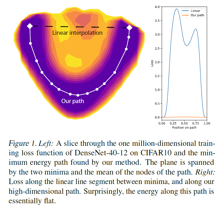
Now we are more interested in a group of studies in which it is proved that between two minima in the space of weights $$$\ theta_1$ and $$$\ theta_2$ it is almost always possible to draw a certain curve, throughout which the loss function will not exceed $$$\ max (E (\ theta_1), E (\ theta_2)) + \ epsilon$ for $$$\ epsilon$ , separated from zero by a certain limit, but much smaller than the typical values ​​of the loss function [17] [18] [19]. There are several ways at once to form such a curve: as a rule, they have a simple segment between $$$\ theta_1$ and $$$\ theta_2$ is divided into links, after which the nodes connecting them are moved by gradient descent in the space of weights. Using such curves, one can, for example, assemble better network assemblies [18]. Their results show that the cluster of minima has a “porous” structure.



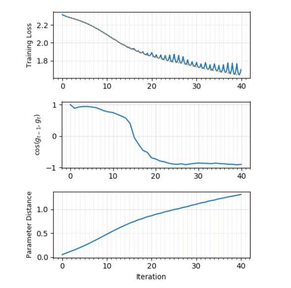
A very recent article from an international team of scientists [23] goes to the same piggy bank, in which they build loss loss charts between $$$\ theta_ {t}$ and $$$\ theta_ {t + 1}$ and the angle between the directions of the gradient at times $$$t$ and $$$t + 1$ . It turns out that at the beginning of training, the gradients of neighboring steps are directed approximately in one direction and the error function decreases monotonically, but from a certain point in time $$$E (\ theta)$ in between $$$\ theta_ {t}$ and $$$\ theta_ {t + 1}$ begins to show characteristic minima, and the angle between the gradients tends to ~ 170 degrees. Indeed, it is very likely that the gradient descent “bounces off” the walls of the “saddle” with a small slant! The picture is much cleaner when gradient descent is carried out using the entire dataset; The use of minibatch distorts the picture beyond recognition, which is logical. The learning rate does not affect the angle chart, but the size of the batch is very much the same. The intersection of local minima, the researchers found.



Until now, we believed that the quality of the minimum found depends only on its depth. However, many researchers note that the width of the minimum also matters. Formally, it can be defined in different ways; I will not give different formulations (see [20], if you still want to see them), then it is enough to understand the basic idea. Here is an illustration:



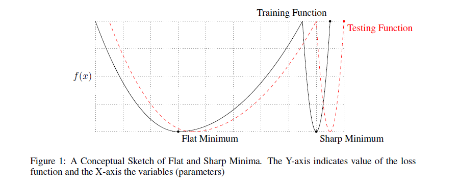
The minimum of black graphics on the left is wide, on the right is narrow. Why does it matter? The distribution of training data does not exactly coincide with the distribution of test data. It can be assumed that the minimum $$$E ^ {*} (\ theta)$ on the test data will look slightly different from the minimums of the original function $$$E (\ theta)$ , in particular, $$$\ theta$ minimums are likely to be shifted relative to each other. But if such a distortion is not terrible for a wide minimum, then a narrow one may change beyond recognition. Again, look at the picture above. If you accept that the black graph is the original $$$E (\ theta)$ , and red is a test one, then you can immediately see what problems this can lead to.

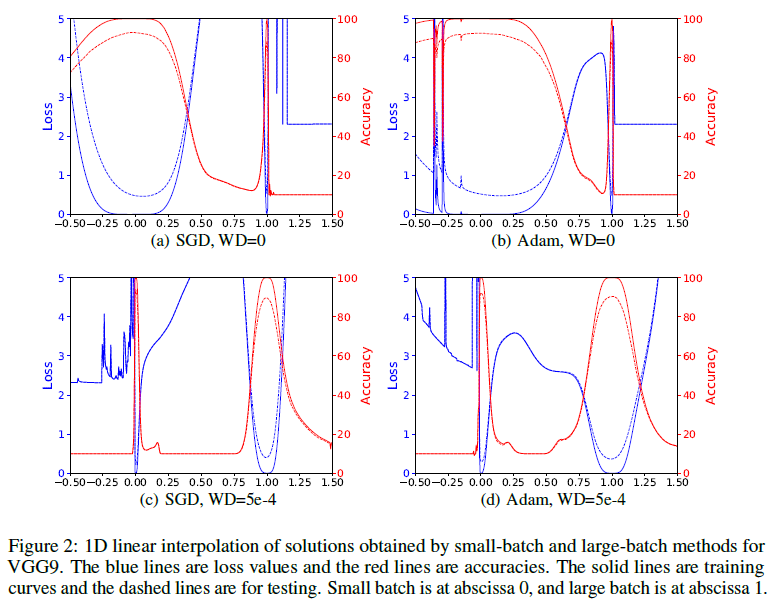
It has been observed in practice that gradient descent with large batch systematically achieves slightly better results in the training sample, but loses on the test one. This is often due to the fact that small batch'i make noise in the assessment of the target distribution and do not allow to settle $$$\ theta$ in a narrow minimum [21]. Approximately the same thing happens as in the picture above: the function is constantly changing (this time intentionally), and crests form at the place of the hollows. From narrow depressions with such a "stir" $$$\ theta$ thrown out, but not from the wide ones. Also, the authors [21] claim that when learning with a small subsample size $$$\ theta$ runs away significantly farther from the point of initialization than otherwise. Such an indicator is described by the term “research ability of the gradient descent algorithm,” and is also considered favorable for achieving good results.

Alas, not so simple. We are faced with the problem mentioned above: the width of the minimum depends on the parameterization [20]. In networks with ReLu-activations, it is enough just to build an example when two sets of weights $$$\ theta_1$ and $$$\ theta_2$ represent essentially the same network but $$$\ theta_1$ - narrow minimum, and $$$\ theta_2$ - wide.A more specific example can be seen in [13], where narrow and wide minima on the loss interpolation graph change places when regularization is turned on:



Perhaps this is the reason for the very modest success of the SGD modification, aimed at directing optimization to wide troughs [ 22]. Very famous scientists demonstrate plausible histograms of the Hessians, but the gain in quality remains almost imperceptible.

Cross comparison

So what do we have?



The theoretical work of Chromanska [5], Kawaguchi [8] and Yun [14] are consistent with each other. Linear neural networks are a simple special case, and it is quite logical that instead of the inner zone of a complex landscape we get one net global minimum (despite the fact that there is a “saddle zone” there and there). In [14], much stronger conditions on the input function are specified.

The connection of theory with practice:

1. Chromanska's statements about the complex landscape in the subspace of minima are consistent with the work on the construction of low-energy curves between the minima $$$E(\theta)$ [17][18][19], , , c snapshot-[24]. [19] , «» , — [5].
2. Chromanska «» , , [3]: loss'.
3. [23], «» .
4. ( loss' ?), , [25]. , / .
5. [12] [11], [8] [14], residual learning , [13].
6. , SGD , Adam [26][27]. SGD , . , 100 , 100 . , , , .
7. , , . «» : -, « » , , [19], -, [32] ( [31]), -, , [33]. (optimal brain damage, ).

In my opinion, the statement that it is not worthwhile to look for a global minimum remains unproved, because it will have the same generalizing ability as the local minima scattered around it. Empirical experience suggests that networks obtained by different launches of the same minimizer make errors on different elements (see dissonance graphs, for example, in [16] or in any work on network ensembles). The same is said of the work on the analysis of the learned features. In [25], the point of view is defended that most of the most useful features are consistently learned, but some of the auxiliary ones are not. If you put together all the rarely appear filters, should it get better? Again we recall the ensembles consisting of different versions of the same model [24] and the redundancy of weights in the neural network [28]. It inspires confidencethat still somehow you can take the best from each model launch and greatly improve the predictions without changing the model itself. If the landscape in a bunch of minima is really incorrigibly impassable for gradient descent, it seems to me that after reaching it you can try switching from SGD to evolutionary strategies [31] or something like that.

However, this is also only unsubstantiated thoughts. Perhaps, really, you should not look for a black cat in a black million-dimensional hyperspace, if it is not there; that it is foolish to fight for the fifth decimal places in the high. A clear awareness of this would give the scientific community an impetus to focus on new network architectures. ResNet went well, why can't you think of something else? Also do not forget about the pre-and post-processing data. If you can convert$$X , in order to "bare" the distribution fold to be laid, then you should not neglect it. In general, it is worth reminding once again that “to find the global minimum of the loss function”$X$

$$≠ “get a good working network out”. In pursuit of the global minimum, it is very easy to retrain the network to a state of complete incapacity [35]. Where, in my opinion, should the community of scientists move on?$\neq$

1. We need to try new modified gradient descent methods that are well able to cross the terrain with saddle points. Preferably, the methods of the first order, with the Hessian any fool can. There are already works on this topic with pretty-looking graphs [29] [30], but there are still many low-hanging fruits in this area of ​​research.
2. I would like to know more about the subspace of minima. What are its properties? Is it possible, having received a sufficient number of local minima, to estimate where the global one will be, or at least a higher-quality local one?
3. Theoretical studies are concentrated mainly on L2-loss. It would be interesting to see how cross-entropy affects the landscape.
4. The situation with wide / narrow minima is unclear.
5. The question remains about the quality of the global minimum.

If there are students among readers who will soon defend a diploma in machine learning, I would advise them to try the first task. If you know which way to look, it is much easier to come up with something healthy. It is also interesting to try to replicate the work of LeCun [34], varying the input data.

On this I have everything. Follow the events in the scientific world.

Thanks to asobolev from the Open Data Science community for a productive discussion.

Bibliography

[1] Blum, AL and Rivest, RL; Training a 3-node neural network is np-complete; 1992
[2] Saxe, McClelland & Ganguli; Exact solutions to deep linear neural networks; 19 Feb 2014. (305 quotes on Google Scholar)
[3] Yann N. Dauphin et al; Identifying and attacking the saddle point problem in high-dimensional non-convex optimization; Jun 10, 2014 (372 Cyats on Google Scholar, pay attention to this article)
[4] Alan J. Bray and David S. Dean; Gaussian fields on large-dimensional spaces; 2007
[5] Anna Choromanska et al; The Loss Surfaces of Multilayer Networks; 21 Jan 2015 (317 quotes on Google Scholar, pay attention to this article)
[6] Anna Choromanska et al; Multiple Networks; 2015
[7] Grzegorz Swirszcz, Wojciech Marian Czarnecki & Razvan Pascanu; Local Minima in Training of Neural Networks; 17 Feb 2017
[8] Kenji Kawaguchi; Deep Learning Without Poor Local Minima; 27 Dec 2016. (70 quotes at Research Gate, pay attention to this article)
[9] Baldi, Pierre, & Hornik, Kurt; Neural networks and principal component analysis: Learning from examples without local minima; 1989.
[9] Haihao Lu & Kenji Kawaguchi; Depth Creates No Bad Local Minima; 24 May 2017.
[11] Moritz Hardt and Tengyu Ma; Identity matters in deep learning; 11 Dec 2016.
[12] A. Emin Orhan, Xaq Pitkow; Skip Connections Eliminate Singularities; 4 Mar 2018
[13] Hao Li, Zheng Xu, Gavin Taylor, Christoph Studer, Tom Goldstein; Visualizing the Loss Landscape of Neural Nets; 5 Mar 2018 (pay attention to this article)
[14] Chulhee Yun, Suvrit Sra & Ali Jadbabaie; Global Optimality Conditions for Deep Neural Networks; Feb 1, 2018 (pay attention to this article)
[15] Kkat; Fallout: Equestria; 25 Jan, 2012
[16] Daniel Jiwoong Im, Michael Tao and Kristin Branson; An Empirical Analysis of the Deep Network Loss Surhaces.
[17] C. Daniel Freeman; Topology and Geometry of Half-Rectified Network Optimization; 1 Jun 2017.
[18] Timur Garipov, Pavel Izmailov, Dmitrii Podoprikhin, Dmitry Vetrov, Andrew Gordon Wilson; Loss Surfaces, Mode Connectivity, and Fast Ensembling of DNNs; 1 Mar 2018
[19] Felix Draxler, Kambis Veschgini, Manfred Salmhofer, Fred A. Hamprecht; Essentially No Barriers in Neural Network Energy Landscape; 2 Mar 2018 (pay attention to this article)
[20] Laurent Dinh, Razvan Pascanu, Samy Bengio, Yoshua Bengio; Sharp Minima Can Generalize For Deep Nets; 15 May 2017
[21] Nitish Shirish Keskar, Dheevatsa Mudigere, Jorge Nocedal, Mikhail Smelyanskiy and Ping Tak Peter Tang; On Large-batch Training for Deep Learning: Generalization Gap and Sharp Minima; 9 Feb 2017
[22] Pratik Chaudhari, Anna Choromanska, Stefano Soatto, Yann LeCun, Carlo Baldassi, Christian Borgs, Jennifer Chayes, Levent Sagun, Riccardo Zecchina; Entropy-SGD: Biasing Gradient Descent into Wide Valleys; 21 Apr 2017
[23] Chen Xing, Devansh Arpit, Christos Tsirigotis, Yoshua Bengio; A Walk with SGD; 7 Mar 2018
[24] habrahabr.ru/post/332534
[25] Yixuan Li, Jason Yosinski, Jeff Clune, Hod Lipson, & John Hopcroft; Convergent Learning: Do Different Neural Networks Learn the Same Representations? 28 Feb 2016 (pay attention to this article)
[26] Ashia C. Wilson, Rebecca Roelofs, Mitchell Stern, Nathan Srebro and Benjamin Recht; The Marginal Value of Adaptive Gradient Methods in Machine Learning
[27] shaoanlu.wordpress.com/2017/05/29/sgd-all-which-one-is-the-best-optimizer-dogs-vs-cats-toy-experiment
[28] Misha Denil, Babak Shakibi, Laurent Dinh, Marc'Aurelio Ranzato, Nando de Freitas; Predicting Parameters in Deep Learning; Oct 27, 2014
[29] Armen Aghajanyan; Charged Point Normalization: An Efficient Solution to the Saddle Point Problem; 29 Sep 2016.
[30] Haiping Huang, Taro Toyoizumi; Reinforced stochastic gradient descent for deep neural network learning; 22 Nov 2017.
[31] habrahabr.ru/post/350136
[32] Quynh Nguyen, Matthias Hein; The Loss Surface of the Deep and Wide Neural Networks; 12 Jun 2017
[33] Itay Safran, Ohad Shamir; Basin in Overspecified Neural Networks; 14 Jun 2016
[34] Levent Sagun, Leon Bottou, Yann LeCun; Eigenvalues of the Hessian in Deep Learning: Singularity and Beyond; 5 Oct 2017
[35] www.argmin.net/2016/04/18/bottoming-out
Source: https://habr.com/ru/post/351924/