Quantum circuits and valves - introductory course
We continue the cycle of quantum articles. Today we dive into the formulas and understand how you can manipulate qubits - elementary computational units. In addition, consider the principles of chains and algorithms. More under the cut!

The goal of this article is to help you quickly get acquainted with the basic principles of operation of quantum gates and understand how these gates are combined into chains that clearly represent quantum algorithms (some of which we will discuss in subsequent publications).
')
For your convenience, I will publish a summary of all the most important gates, circuit elements, etc. from the articles of this series in the form of a cheat sheet (so that you do not have to search for the necessary information for a long time). In my future articles, it will be called "Quantum Computing: A Brief Reference."
Let's start with the basics - with the notation of some common quantum states, which we will subsequently manipulate:

All of them are pure single-qubit states, so they can be represented as points on the Bloch sphere:

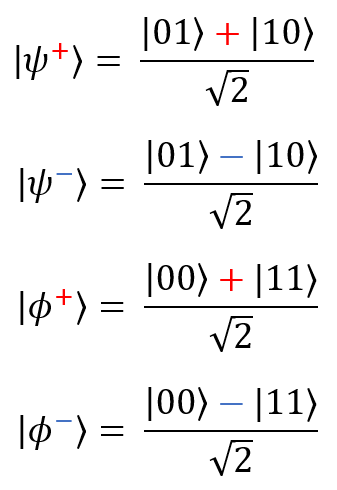
Now - the four states of Bell (they are also called ESR pairs, in honor of Einstein, Podolsky and Rosen - they are the authors of the ideas that Bell later developed). These are the simplest examples of the quantum entanglement of two qubits:
Finally, we will use the so-called GHC states (Greenberg – Horn – Zeilinger). Here is their general form (for n qubits) and the simplest form (for three qubits):
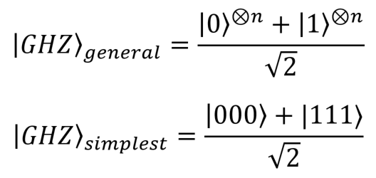
The Bell states and the GHC states are very important because their behavior is completely different from the predictions of the classical theory due to the level of entanglement in such systems (this principle of “maximum entanglement” will be discussed in a subsequent publication).
Angles of rotation in the theory of quantum computing are measured in radians. A full circle (360 °) corresponds to 2π radians. Angles are measured counterclockwise. The values of the most important angles in degrees and in radians are shown below.

Before you delve into the study of quantum gates, you should learn the basics of constructing quantum circuit diagrams (this does not take much time):
Here are the designations of the most important elements:

For more information, see the documentation here and in the book “Quantum Information and Quantum Computations” by M. Nielsen and I. Chang.
Single-qubit gates are naturally the simplest, so we start with them. The operation performed by any one-qubit gate can be represented as a rotation of the vector characterizing the qubit state to another point of the Bloch sphere (see below).
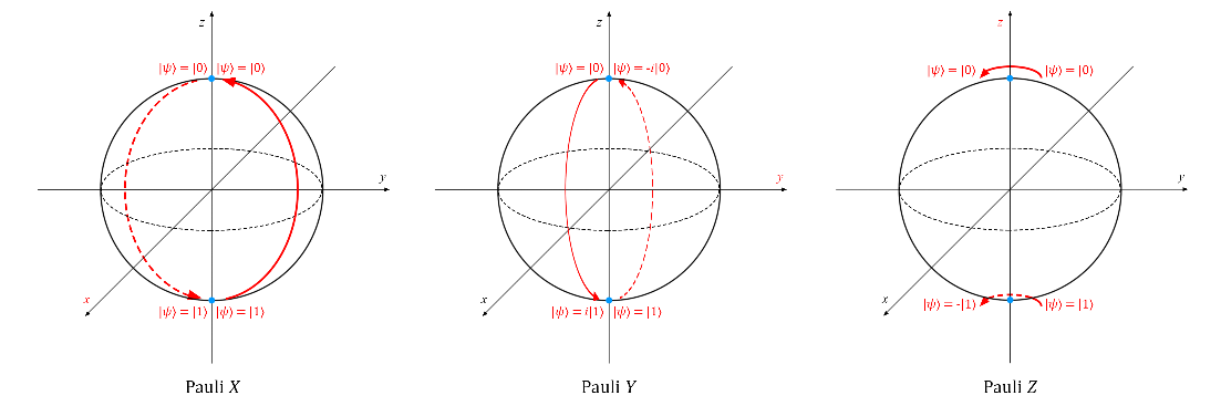
The most elementary one-qubit valves are Pauli X, Y and Z valves:
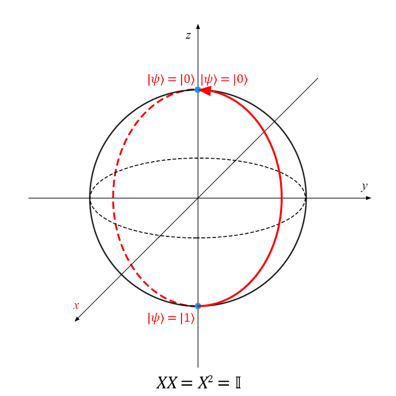
Gate X is very similar to the classic NOT gate: it converts | 0〉 into | 1, and | 1 into | 0. This operation is equivalent to rotating the vector on the Bloch sphere around the x axis by π radians (or 180 °).
The gate Y is expected to correspond to the rotation of the vector around the y axis by π radians. As a result of this operation, the vector | 0〉 turns into i | 1, and | 1〉 - into -i | 0.
Valve Z is a special case of a phase shift valve. (see below) with phi = π = 180 °. It corresponds to the rotation of the vector around the z axis by π radians. It leaves the vector | 0 unchanged, and | 1〉 converts to - | 1.
The work of these transformations is illustrated below with the help of the Bloch sphere (the axis of rotation is highlighted in red in each case; you can click on the image to enlarge it):
It is important to note that after double use of the same Pauli gate to the qubit, it will transition to the initial state (because after rotating the vector by 2π radians or 360 ° around any axis, it will transition to the initial position). Consequently,

Insofar as etc.,
etc.,
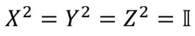
Here II is the designation of the unit matrix: . A unit matrix is called, the result of multiplying which by an arbitrary matrix M (II) is equal to the matrix M: MII = IIM = M. The unit matrix corresponds to a quantum operation that does not change the quantum state. On the Flea field, it looks like this:
In view of this relationship, it is said that the Pauli matrix squared equals the identity matrix.
Below is a description of a few more important single-qubit gates.
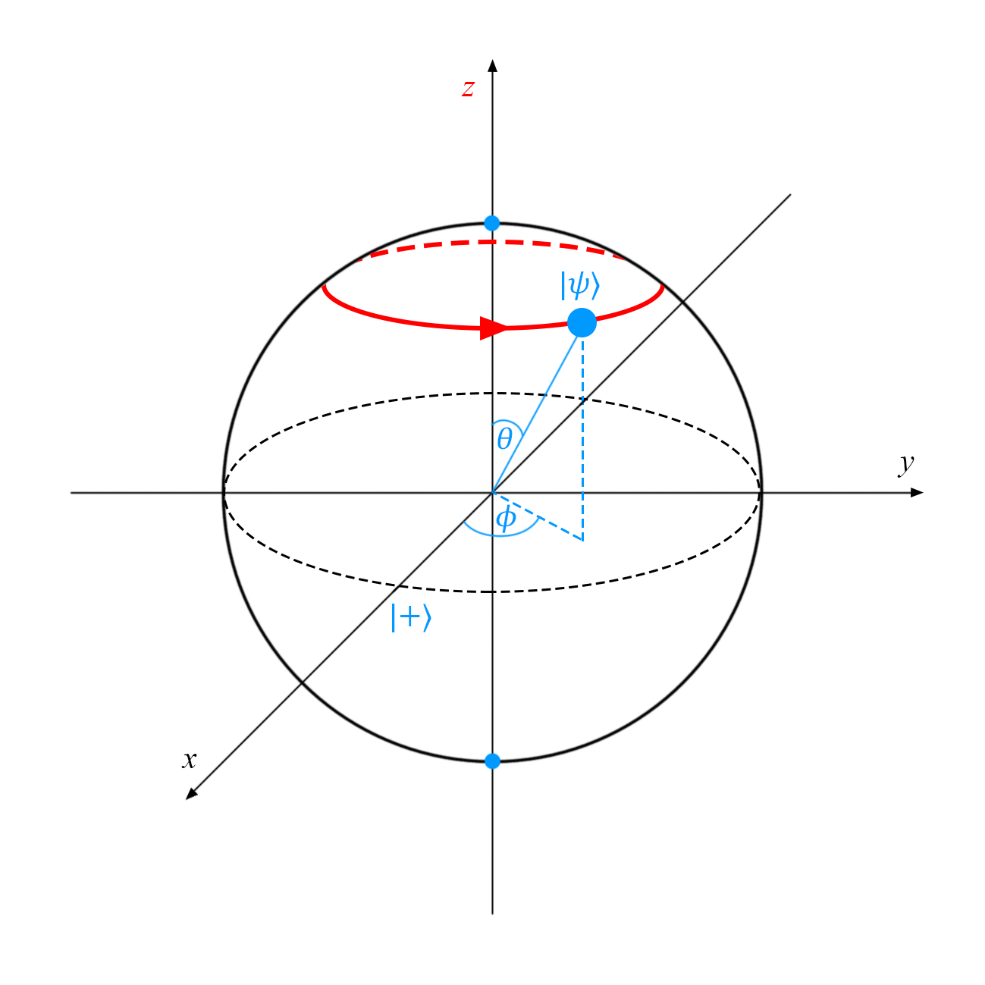
The Hadamard gate is especially important because it can be used to create a superposition of states | 0〉 and | 1〉. This operation is easiest to visualize with the help of the Bloch sphere as a rotation around the x axis by π radians (180 °) with a subsequent rotation around the y axis (clockwise) by π / 2 radians (90 °):

The phase transition valve is a fairly general operation, which has many useful applications. The most common variations are the phase shift valves by π / 4, π / 8 and the Pauli gate Z, for which the parameter fi is π / 2, π / 4 and π, respectively. Phase Shift Example on the field of Flea:
Multi-qubit valves perform operations on two or more qubits. One of the simplest examples is the SWAP valve:
The SWAP gate swaps two input qubits. For example, SWAP | 0〉 | 1 = | 1〉 | 0〉, and SWAP | 0 | 0 = | 0〉 | 0 (the full truth table is listed in the cheat sheet).
Another class of multi-bit valves is the so-called controlled valves. At least one control and one controlled qubit are fed to the input of any controlled valve, and the valve will perform the operation on the controlled qubit only if the controlling qubit is in a certain state.
Gates that perform an operation with a control qubit | 1 are indicated by a filled circle on the wire of the control qubit. Gates that perform an operation with a control qubit equal to | 0 are indicated by an empty circle, as shown below.

In order to compose the matrix of any control valve, you need to add a unit matrix in the upper left corner of the matrix of the desired valve, and fill all other cells with zeros. Here is an example:
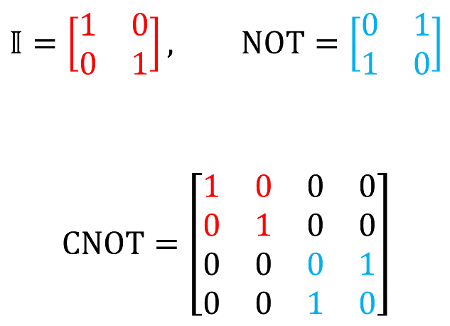
Regular gates in Q # can be converted to control using the Controlled keyword, as described here (in the “Controlled” section at the very bottom of the page). For example, the CNOT gate (recall that the NOT gate is equivalent to the Pauli X-gate) can be obtained with the command
where [control] is an array of input control qubits.
Other common controlled valves are described below (we selected the identity matrix in red and the source valve matrix in blue, as above):
As we mentioned in the previous publication , regardless of the physical system we use to simulate a quantum computer, it must be possible to implement a “universal set” of gates. This means that any valid computational operation in our system must be transformable to a finite sequence of known gates. Here is an example of such a universal set: Hadamard valve, phase shift valve, CNOT valve and π⁄8 valve.
The property of universality is much more interesting than it might seem at first glance. If there is a universal set of gates in a quantum computer, then any transformation allowed by the laws of quantum physics can be realized with its help. This means that with the help of the universal set you can not just execute any quantum program, but simulate any physical phenomenon. Therefore, the universality property allows using quantum computers to model molecules, superconductors, and any strange and beautiful quantum systems. This feature of quantum computers allows you to simulate physical phenomena, which in the long term will allow quantum systems to exceed the potential of the most powerful supercomputers. Already not boring, right?
With the help of these (and some other) major gates, it is already possible to create fully functional quantum chains! In the next publication I will explain how using this newly acquired knowledge one can realize the quantum Fourier transform - a very important operation, which has a great many practical applications.
Articles from the cycle:
Introduction
The goal of this article is to help you quickly get acquainted with the basic principles of operation of quantum gates and understand how these gates are combined into chains that clearly represent quantum algorithms (some of which we will discuss in subsequent publications).
')
For your convenience, I will publish a summary of all the most important gates, circuit elements, etc. from the articles of this series in the form of a cheat sheet (so that you do not have to search for the necessary information for a long time). In my future articles, it will be called "Quantum Computing: A Brief Reference."
Basics: Quantum States
Let's start with the basics - with the notation of some common quantum states, which we will subsequently manipulate:
All of them are pure single-qubit states, so they can be represented as points on the Bloch sphere:
Now - the four states of Bell (they are also called ESR pairs, in honor of Einstein, Podolsky and Rosen - they are the authors of the ideas that Bell later developed). These are the simplest examples of the quantum entanglement of two qubits:
Finally, we will use the so-called GHC states (Greenberg – Horn – Zeilinger). Here is their general form (for n qubits) and the simplest form (for three qubits):
The Bell states and the GHC states are very important because their behavior is completely different from the predictions of the classical theory due to the level of entanglement in such systems (this principle of “maximum entanglement” will be discussed in a subsequent publication).
Basics: radians
Angles of rotation in the theory of quantum computing are measured in radians. A full circle (360 °) corresponds to 2π radians. Angles are measured counterclockwise. The values of the most important angles in degrees and in radians are shown below.
Basics: Quantum Chain Diagrams
Before you delve into the study of quantum gates, you should learn the basics of constructing quantum circuit diagrams (this does not take much time):
- Time on the quantum diagram moves from left to right.
- Each qubit corresponds to a single horizontal line.
- Valves are usually indicated by squares. The type of valve is indicated by letters or other symbols in this box (there are exceptions to this rule. Usually, these are qubit valves that have classical analogs (for example, the NOT gate)).
- Some valves may correspond to several chart elements (for example, the NOT gate).
- As a result of measuring a qubit, all superpositions collapse, the quantum properties of a qubit disappear, and it turns into a normal bit. Therefore, we can assume that the measuring element (shown below) takes the qubit as input and outputs the classic bit. This operation in the Q # language corresponds to the Measure command (bases: Pauli [], qubits: Qubit []) or M (qubit: Qubit) on the bottom of Z.
Here are the designations of the most important elements:
For more information, see the documentation here and in the book “Quantum Information and Quantum Computations” by M. Nielsen and I. Chang.
Single-qubit valves
Single-qubit gates are naturally the simplest, so we start with them. The operation performed by any one-qubit gate can be represented as a rotation of the vector characterizing the qubit state to another point of the Bloch sphere (see below).
The most elementary one-qubit valves are Pauli X, Y and Z valves:
| Titles | Matrix representation | Legend | Q # presentation |
|---|---|---|---|
Pauli gate X, X, NOT, bit switching,  | 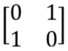 |   | X (qubit: Qubit) |
Pauli valve Y, Y,  |  |  | Y (qubit: Qubit) |
Pauli valve Z, Z, phase switching,  | 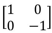 | 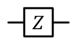 | Z (qubit: Qubit) |
The gate Y is expected to correspond to the rotation of the vector around the y axis by π radians. As a result of this operation, the vector | 0〉 turns into i | 1, and | 1〉 - into -i | 0.
Valve Z is a special case of a phase shift valve.
The work of these transformations is illustrated below with the help of the Bloch sphere (the axis of rotation is highlighted in red in each case; you can click on the image to enlarge it):
It is important to note that after double use of the same Pauli gate to the qubit, it will transition to the initial state (because after rotating the vector by 2π radians or 360 ° around any axis, it will transition to the initial position). Consequently,
Insofar as
etc.,Here II is the designation of the unit matrix:
. A unit matrix is called, the result of multiplying which by an arbitrary matrix M (II) is equal to the matrix M: MII = IIM = M. The unit matrix corresponds to a quantum operation that does not change the quantum state. On the Flea field, it looks like this:In view of this relationship, it is said that the Pauli matrix squared equals the identity matrix.
Below is a description of a few more important single-qubit gates.
| Titles | Matrix representation | Legend | Q # presentation |
|---|---|---|---|
| Hadamard valve, H | 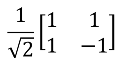 |  | H (qubit: Qubit) |
| Phase shift | 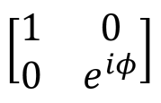 |  | R1 (theta: Double, qubit: Qubit) More generally R (pauli: Pauli, theta: Double, qubit: Qubit) |
Phase shift  S S | 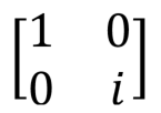 |  | S (qubit: Qubit) |
 , T , T | 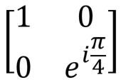 |  | T (qubit: Qubit) |
The phase transition valve is a fairly general operation, which has many useful applications. The most common variations are the phase shift valves by π / 4, π / 8 and the Pauli gate Z, for which the parameter fi is π / 2, π / 4 and π, respectively. Phase Shift Example
Multi-bit valves
Multi-qubit valves perform operations on two or more qubits. One of the simplest examples is the SWAP valve:
| Titles | Matrix representation | Legend | Q # presentation |
|---|---|---|---|
| Swap | 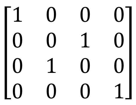 |  | SWAP (qubit1: Qubit, qubit2: Qubit) |
Another class of multi-bit valves is the so-called controlled valves. At least one control and one controlled qubit are fed to the input of any controlled valve, and the valve will perform the operation on the controlled qubit only if the controlling qubit is in a certain state.
Gates that perform an operation with a control qubit | 1 are indicated by a filled circle on the wire of the control qubit. Gates that perform an operation with a control qubit equal to | 0 are indicated by an empty circle, as shown below.
In order to compose the matrix of any control valve, you need to add a unit matrix in the upper left corner of the matrix of the desired valve, and fill all other cells with zeros. Here is an example:
Regular gates in Q # can be converted to control using the Controlled keyword, as described here (in the “Controlled” section at the very bottom of the page). For example, the CNOT gate (recall that the NOT gate is equivalent to the Pauli X-gate) can be obtained with the command
(Controlled X)([control], (target)) where [control] is an array of input control qubits.
Other common controlled valves are described below (we selected the identity matrix in red and the source valve matrix in blue, as above):
| Titles | Matrix representation | Legend | Q # presentation |
|---|---|---|---|
| CNOT | 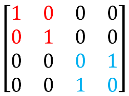 |  | CNOT (control: Qubit, target: Qubit) or (Controlled X) ([control], (target)); |
| CCNOT, Toffoli valve | 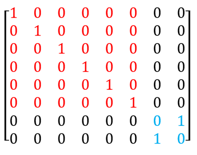 |  | CCNOT (control1: Qubit, control2: Qubit, target: Qubit) or (Controlled X) ([control1; control2], target); |
| CSWAP, Fredkin valve | 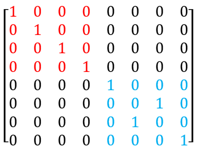 |  | (Controlled SWAP) ([control], (target)); |
Universal kits
As we mentioned in the previous publication , regardless of the physical system we use to simulate a quantum computer, it must be possible to implement a “universal set” of gates. This means that any valid computational operation in our system must be transformable to a finite sequence of known gates. Here is an example of such a universal set: Hadamard valve, phase shift valve, CNOT valve and π⁄8 valve.
The property of universality is much more interesting than it might seem at first glance. If there is a universal set of gates in a quantum computer, then any transformation allowed by the laws of quantum physics can be realized with its help. This means that with the help of the universal set you can not just execute any quantum program, but simulate any physical phenomenon. Therefore, the universality property allows using quantum computers to model molecules, superconductors, and any strange and beautiful quantum systems. This feature of quantum computers allows you to simulate physical phenomena, which in the long term will allow quantum systems to exceed the potential of the most powerful supercomputers. Already not boring, right?
Many more interesting things await us!
With the help of these (and some other) major gates, it is already possible to create fully functional quantum chains! In the next publication I will explain how using this newly acquired knowledge one can realize the quantum Fourier transform - a very important operation, which has a great many practical applications.
Additional resources
Source: https://habr.com/ru/post/351628/
All Articles