Quantum computing and Q # language for beginners
You may have learned about the release of the Quantum Development Kit, a package of quantum tools, and thought it sounded really awesome ... and then you remembered that you almost knew nothing about quantum mechanics. But that's okay. In 30 minutes you will know enough about qubbles, superposition and quantum entanglement to write your first program and, more importantly, to understand well what it does.
Frances is a graduate of Imperial College London with a degree in computational technology. She wrote her graduation project, working in the Microsoft Research division. Frances currently works at Microsoft as a software engineer. Its main areas of activity are machine learning, big data and quantum computing.
If you do not program at the lowest level, then you can completely forget that any programs, in fact, only manipulate the zeros and units that are stored in our "classic" computers. Discrete binary states of physical systems correspond to these zeros and ones. Quantum computers operate with continuous state ranges. In part, their capabilities are due precisely to this.
')
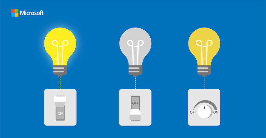
The classic bit can take only one of two states - “on” or “off”, like a normal incandescent lamp. Qubits, the basis of quantum computers, are more like a lamp with adjustable brightness.
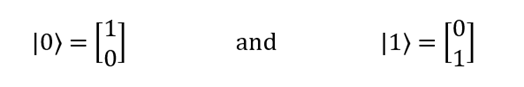
To record two states of qubits, you can use sconces and ket symbols (Dirac symbols) that correspond to the following vectors:
Using a linear combination of these two states, any possible combination of vectors | 0 and | 1 can be expressed. In quantum mechanics, this combination is called a superposition. The corresponding entry in the Dirac notation will look like this:
| ψ⟩ = α | 0〉 + β | 1
The values of α and β are related to probabilities (with one small difference — these coefficients can be expressed by complex numbers). You can think of them as real numbers, but in this case, remember that they can take negative values. However, the sum of their squares is always 1.
Quantum states are a weird thing. As a result of the measurement (or, as they say, “in the presence of an observer”), the qubit collapses immediately. What does it mean? Suppose a qubit is in a superposition state. If you measure it, it will take one specific value - | 0〉 or | 1 (both measurements cannot show both results at once!). After measuring the qubit, the coefficients α and β, which characterized its previous state, will, in fact, be lost.
Therefore, the apparatus of the theory of probability is used to describe the measurements of qubits. In the general case, the probability that a qubit state measurement will show the result | 0〉 is equal to and the probability to get the state | 1〉 is
  . Consider an example. Suppose we have the following qubit:
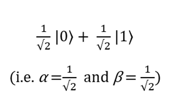
If we measure its state, then in 50% of cases we will get a value of 0, because:
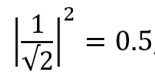
That is, after the measurement, it will be in the state | 0〉 (that is, α = 1, β = 0). For the same reason, the probability of getting state 1 is 50%. In this case, after the measurement, the qubit will move to the state | 1 (that is, α = 0, β = 1).

For the first time, all this is very confusing (nothing will change for the second, third and fourth time). The basic idea here is that probabilistic quantum states can be used for calculations, and in some cases this quantum “strangeness” allows us to obtain systems with efficiency higher than the classical ones. Now let's see how these qubits can be used for computations, like the classic bits.
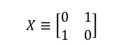
Let's go back to the more familiar things. In the classical theory of computation, logic gates are used to perform operations on bits. Qubit manipulations use similar constructions - quantum gates. For example, the NOT gate performs transformations 0 → 1 and 1 → 0. The quantum gate NOT is similar to its classical ancestor: it performs transformations | 0〉 → | 1〉 and | 1 → | 0. This means that after passing such a valve, the qubit from the state α | 0〉 + β | 1〉 changes to the state α | 1〉 + β | 0. The gate NOT can be written in the form of a matrix (X), which swaps 0 and 1 in the state matrix:
As you can see, X | 0〉 = | 1, and X | 1 = | 0:
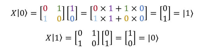
Since | 0〉 and | 1〉 in vector form are written as and
and  , the first column of the matrix X can be considered as a transformation of the vector | 0, and the second - as a transformation of the vector | 1.
It would seem that the difference from the classical case is not so great. But do not forget what we said in the previous section: measuring the state of a qubit is probabilistic in nature. As is known from elementary probability theory, the sum of the probabilities of the complete group of incompatible events is equal to one. therefore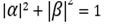 for the quantum state, α | 0〉 + β | 1〉.
It follows that not all imaginable gates can exist in the quantum world. Here is one of the limitations: the condition for the normalization of the quantum state of a qubit, , must be observed both before the passage of the valve and after it. In terms of matrix algebra, this condition will be satisfied if the matrix is unitary.
I will try to explain what the mathematical concept of unitarity means. If you read it quickly enough, you just find yourself on the next sentence. A valve is called unitary if obtained by transposition and complex conjugation
  and is the unit matrix of rank 2. If we speak in human language, this means that the transformation does not change the length of the vector. If the vector length does not change with time, then the sum of all probabilities is invariably equal to one, or 100% (as it should be). The calculations, as a result of which the sum of all probabilities turns out to be equal to 200% or 25%, would be meaningless. Unitary matrices protect at least from such insanity (although it remains abundant in the quantum world).
Good news: this restriction is the only one. Due to this condition, some classical gates do not have a quantum analogue, however, some quantum gates do not have a classical prototype. Next we analyze the most important of the quantum gates.
The valves described below will be used in our first quantum program, so try to memorize them. The Z valve works very simply: it saves the component | 0 and changes the sign of the component | 1. It can be written as a matrix

which transforms the states of qubits as follows: | 0〉 → | 0〉, | 1〉 → - | 1〉 (remember that the first column of the matrix describes the transformation of the vector | 0, the second - the transformation of the vector | 1).
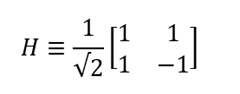
The Hadamard gate creates a superposition of states | 0〉 and | 1, similar to those discussed above. Its matrix notation looks like this:
which corresponds to the following state transformations of qubits: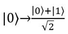 ,
, 
More detailed information on unitary matrices and on how to visualize valves is provided in the resources referenced in the "Additional materials" section.
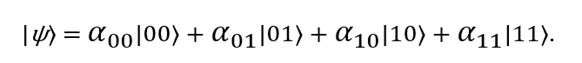
Consider something more familiar. Classical bits exist not only singly, but also in the form of combinations: for example, 00, 01, 10 and 11. In quantum computing, similar combinations are used: | 00〉, | 01〉, | 10 and | 11〉. The state of two qubits can be described using the following vector:
As before, the probability to receive as a result of measurement the value 00 is equal ,
,
for 01, the probability is etc.
etc.
Suppose now that we want to measure the state of not both qubits, but only the first one. The probability of getting 0 is equal to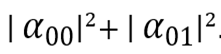 . As we remember, measurement changes state, therefore after it the vector will matter

Pay attention to the numerator: we removed all the terms for which the first bit is 1 (since, by hypothesis, the measurement result is 0). In order for a vector to describe an admissible quantum state, it is necessary that the square of the sum of amplitudes be equal to one (both before and after the transformation). In order for this condition to be satisfied, we add the normalization factor — the reciprocal of the square root of the determinant.
We have already disassembled the operation of the NOT gate. Next in line is the CNOT (controlled-NOT, “NOT controlled”) gate. At its entrance serves two qubits. The first is called the manager, the second - managed. If the controlling qubit is | 0, then the state of the controlled qubit does not change. If the controlling qubit is | 1, then the operation NOT is applied to the managed qubit.
The CNOT operation can be interpreted in several ways. Like the valves X, Z and H, it can be written in matrix form, which is denoted by the letter U.
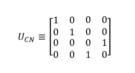
You can see that the columns of the matrix correspond to the following transformations: | 00〉 → | 00〉, | 01〉 → | 01, | 10 → | 11, | 11〉 → | 10. Like the matrices that we sorted out , it is unitary, which means
  .
.
Also for this valve the following designation is used (the upper part corresponds to the control qubit, the lower part - to the controlled one):

Looks like an exhibit of the exhibition of contemporary art.
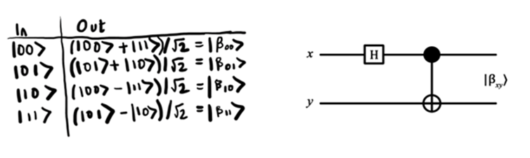
This important topic is worth devoting a whole section. In total there are four states of Bell. One of them (| ϕ +⟩) will be used in the quantum program below. Let's consider it.
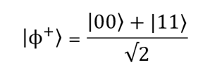
Suppose we measure the state of the first qubit. Result | 0〉 we get with probability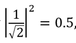 . This means that the state after the measurement | ψ '⟩ = | 00〉, or | 1 with the same probability (0.5), and the state after the measurement | ψ' = | 11. For the curious we cite the complete set of Bell states (they represent the simplest cases of quantum entanglement):

Now suppose that we measured the state of the second qubit. According to the same reasoning, after measuring the steam will be in the state | 00〉 or | 11. If after this we decide to measure the state of the first qubit, the probabilities will no longer be equal to 0.5. We will get | 0〉 with a probability of 1 or 0, depending on what the measurement result was. Here it is important to understand that these results are related. The first to notice this were Albert Einstein, Boris Podolsky and Nathan Rosen (therefore, these states are sometimes called “EPR pairs”). Subsequently, their theory was developed by John Bell.
One final observation: Bell states can be generated using the Hadamard valve and the CNOT valve. In my opinion, it is admirable. Hadamard's gate puts the first qubit into a superposition state. Then this qubit is fed to the control input of the CNOT valve. Here is how this process can be represented using a circuit diagram:
To learn more about how each of these transformations works, refer to the additional materials (the list is given below). We already know about qubit states, quantum gates and Bell states enough to write our first program using qubits.
We will follow the instructions from the documentation .
This tutorial will help you do the following: install a quantum software development package (steps 1–2), select a qubit and perform a number of simple manipulations on it — for example, set it to a certain state and measure it (steps 3–5), then translate the qubit is in the superposition state (step 6), and after that the two qubits are transformed into an entangled state - the Bell state, or the EPR pair (step 7).
It is recommended that you follow the instructions in the manual referenced above and return to this material if you need tips or additional explanations.
Q # is at the bottom of this list.

We followed this advice, but this is not necessary, especially if you like to take risks.
This operation converts our qubit to the selected (by us) state - 0 or 1. First, we measure the qubit (this operation is denoted by the letter M), and it collapses into the state 0 or 1. If the measured state does not match the desired state, we change it with the help of the valve NOT, X. Otherwise, nothing needs to be done.
This small piece of code is intended to test the operation we just wrote. This is a very simple program: it checks that the qubit has been transferred to the state we need.
To do this, it takes a measurement in a cycle and counts the number of results 1 using the variable numOnes.
The entry “Qubit [1]” means “create an array of qubits from one element”. The array elements are indexed from scratch. To select two qubits (later we need to do this), we need to write “Qubit [2]”. Cubits in such an array correspond to numbers 0 and 1.
In the for loop, we set the qubit allocated for a certain initial state — One or Zero (in the Driver.cs file, to which we will soon move on, this is done explicitly). We measure this state, and if it is One, we increase the value of the counter by one. The function then returns the number of observed states One and Zero. At the end, the qubit is placed in the Zero state (just to leave it in some known state).
This driver creates a quantum simulator and an array of initial values that need to be checked (Zero and One). Then the simulation is repeated 1000 times, and the result for debugging is displayed on the screen using the System.Console.WriteLine function.
If everything is in order, the display should look like the one shown above. This result means that if we transfer the initial qubit to the Zero state and perform a thousand repetitions, then the number of states | 0〉 according to the observation results will be 1000. The same should be done for the One state.
Let's try something more interesting. Here we change the state of the qubit using the NOT gate.
Then we run the program again and see that the results are reversed.
Then the NOT valve is replaced with the Hadamard valve (H). As a result, as we know, the qubit will go over to the superposition of states, and the result of its measurement can be equal to both | 0〉 and | 1, with some probability.
If you run the program again, we get a rather interesting result.
The number of measurement results | 0〉 and | 1〉 will be approximately equal.
We will now create the state of Bella. Examine the code below. First, we create an array of two qubits (Qubit [2]). The first qubit (in the previous circuit diagram, it was denoted by the symbol x) we transfer to some initial state, and the second one (y in the diagram) is set to the Zero state. This is about the same as entering | 00〉 or | 10〉 depending on X:
According to the diagram, the first qubit, qubits [0], needs to be passed through the Hadamard gate. As a result, he will be in superposition. Then we pass the qubits through the CNOT gate (qubits [0] - the controlling qubit, qubits [1] - controlled) and measure the result.
To understand what result to expect, we repeat once again how our state of Bell works. If we measure the first qubit, we get the value | 0〉 with probability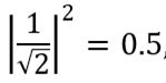 . This means that the state after the measurement | ψ '⟩ = | 00〉 or | 1 with the same probabilities (0.5), and the state after the measurement | ψ' = | 11. Thus, the result of measuring the state of the second qubit will be | 0〉 if the first qubit was in the state | 0, and | 1〉 if the first qubit was in the state | 1. If the states of two qubits were successfully entangled, then our results should show that the first and second qubits are in the same states.
In our code, we check if the measurement result of qubits [1] is equal to the measurement result of qubits [0], using the if operator.
Before checking the results, you need to make another change to the Driver.cs file: add the variable agree.
Now the program can be run. What do these results mean? If the first qubit was initially placed in the Zero state (that is, we input the value | 00), then the Hadamard valve puts the qubits in the superposition state, and the measurement result is | 0 in 50% of cases and | 1 in 50% of cases . The fulfillment of this condition can be estimated by the number of zeros and ones. If the measurement of the state of the first bit did not affect the state of the second, it would remain equal to | 0, and consistency would be achieved only in 499 cases.
But, as we can see, the states of the first and second qubit are completely consistent: the number of results | 0〉 and | 1 (approximately) coincide. Thus, the results are consistent in each of the 1000 cases. This is how Bell states should work.
On it we will finish. You wrote your first quantum program and (since you got to the end), you probably understood what it was doing. It is worth noting a good cup of tea.

There are many examples available in the GitHub repository.
In the next article we will talk about the theory of quantum teleportation and study sample code.
Quantum vents are discussed in more detail in Anita’s blog (note: Anita is simply amazing).
If you want to delve into the topics covered, below is a list of resources that were very helpful to us. The first of them is the book “Quantum Computations and Quantum Information” (M. Nielsen, I. Chang). The second is the Microsoft SDK documentation .
If it will be interesting to readers (leave a comment!), We can make a separate publication about other resources.

Bell states can be generated using the Hadamard valve and the CNOT valve. Hadamard's gate puts the first qubit into a superposition state. Then this qubit is fed to the control input of the CNOT valve. On the circuit diagram, it looks like this:
Let us begin with the first case when a pair of qubits in the state | 00 is input. The first qubit, | 0〉, passes through the Hadamard valve and turns into . The second qubit does not change. Result:
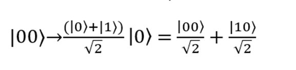
Then the qubits pass through the CNOT gate (which performs the | 00〉 → | 00〉 and | 10〉 → | 11〉) transformations. Now their state will be described by the formula

Second case: Qbits | 01〉 are input. Hadamard's gate puts the first qubit | 0 into the state . The second qubit does not change. Result:
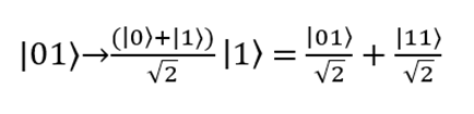
Now we will pass the qubits through the CNOT gate, which performs the transformations | 01〉 → | 01 and | 11 → | 10. The final state of a pair of qubits will look like this:

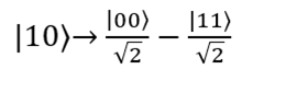
The third case: Qbits | 10 are input. Hadamard's gate puts the first qubit | 1⟩ into the state . The second qubit does not change. Result:

Then the qubits pass through the CNOT gate (which performs the | 00〉 → | 00〉 and | 10〉 → | 11〉) transformations. Now their state will be described by the formula
The fourth case: Qbits | 11 are fed to the input. Hadamard's gate puts the first qubit | 1⟩ into the state . The second qubit does not change. Result:

Now we will pass the qubits through the CNOT gate, which performs the transformations | 01〉 → | 01 and | 11 → | 10. The final state of a pair of qubits will look like this:

Done, we dismantled all cases.
Articles from the cycle:
Frances is a graduate of Imperial College London with a degree in computational technology. She wrote her graduation project, working in the Microsoft Research division. Frances currently works at Microsoft as a software engineer. Its main areas of activity are machine learning, big data and quantum computing.
The content of the article
- Repeat the basics
- Measure qubit
- Quantum gates
- Important valves
- Several qubits
- Another important valve
- Bella's condition
- Writing a quantum program
- What's next?
- application
- Additional materials
Repeat the basics
If you do not program at the lowest level, then you can completely forget that any programs, in fact, only manipulate the zeros and units that are stored in our "classic" computers. Discrete binary states of physical systems correspond to these zeros and ones. Quantum computers operate with continuous state ranges. In part, their capabilities are due precisely to this.
')
The classic bit can take only one of two states - “on” or “off”, like a normal incandescent lamp. Qubits, the basis of quantum computers, are more like a lamp with adjustable brightness.
To record two states of qubits, you can use sconces and ket symbols (Dirac symbols) that correspond to the following vectors:
Using a linear combination of these two states, any possible combination of vectors | 0 and | 1 can be expressed. In quantum mechanics, this combination is called a superposition. The corresponding entry in the Dirac notation will look like this:
| ψ⟩ = α | 0〉 + β | 1
The values of α and β are related to probabilities (with one small difference — these coefficients can be expressed by complex numbers). You can think of them as real numbers, but in this case, remember that they can take negative values. However, the sum of their squares is always 1.
Measure qubit
Quantum states are a weird thing. As a result of the measurement (or, as they say, “in the presence of an observer”), the qubit collapses immediately. What does it mean? Suppose a qubit is in a superposition state. If you measure it, it will take one specific value - | 0〉 or | 1 (both measurements cannot show both results at once!). After measuring the qubit, the coefficients α and β, which characterized its previous state, will, in fact, be lost.
Therefore, the apparatus of the theory of probability is used to describe the measurements of qubits. In the general case, the probability that a qubit state measurement will show the result | 0〉 is equal to
and the probability to get the state | 1〉 is . Consider an example. Suppose we have the following qubit:If we measure its state, then in 50% of cases we will get a value of 0, because:
That is, after the measurement, it will be in the state | 0〉 (that is, α = 1, β = 0). For the same reason, the probability of getting state 1 is 50%. In this case, after the measurement, the qubit will move to the state | 1 (that is, α = 0, β = 1).
For the first time, all this is very confusing (nothing will change for the second, third and fourth time). The basic idea here is that probabilistic quantum states can be used for calculations, and in some cases this quantum “strangeness” allows us to obtain systems with efficiency higher than the classical ones. Now let's see how these qubits can be used for computations, like the classic bits.
Quantum gates
Let's go back to the more familiar things. In the classical theory of computation, logic gates are used to perform operations on bits. Qubit manipulations use similar constructions - quantum gates. For example, the NOT gate performs transformations 0 → 1 and 1 → 0. The quantum gate NOT is similar to its classical ancestor: it performs transformations | 0〉 → | 1〉 and | 1 → | 0. This means that after passing such a valve, the qubit from the state α | 0〉 + β | 1〉 changes to the state α | 1〉 + β | 0. The gate NOT can be written in the form of a matrix (X), which swaps 0 and 1 in the state matrix:
As you can see, X | 0〉 = | 1, and X | 1 = | 0:
Since | 0〉 and | 1〉 in vector form are written as
and , the first column of the matrix X can be considered as a transformation of the vector | 0, and the second - as a transformation of the vector | 1.It would seem that the difference from the classical case is not so great. But do not forget what we said in the previous section: measuring the state of a qubit is probabilistic in nature. As is known from elementary probability theory, the sum of the probabilities of the complete group of incompatible events is equal to one. therefore
for the quantum state, α | 0〉 + β | 1〉.It follows that not all imaginable gates can exist in the quantum world. Here is one of the limitations: the condition for the normalization of the quantum state of a qubit,
, must be observed both before the passage of the valve and after it. In terms of matrix algebra, this condition will be satisfied if the matrix is unitary.I will try to explain what the mathematical concept of unitarity means. If you read it quickly enough, you just find yourself on the next sentence. A valve is called unitary if
obtained by transposition and complex conjugation and is the unit matrix of rank 2. If we speak in human language, this means that the transformation does not change the length of the vector. If the vector length does not change with time, then the sum of all probabilities is invariably equal to one, or 100% (as it should be). The calculations, as a result of which the sum of all probabilities turns out to be equal to 200% or 25%, would be meaningless. Unitary matrices protect at least from such insanity (although it remains abundant in the quantum world).Good news: this restriction is the only one. Due to this condition, some classical gates do not have a quantum analogue, however, some quantum gates do not have a classical prototype. Next we analyze the most important of the quantum gates.
Important valves: valve Z and Hadamard valve
The valves described below will be used in our first quantum program, so try to memorize them. The Z valve works very simply: it saves the component | 0 and changes the sign of the component | 1. It can be written as a matrix
which transforms the states of qubits as follows: | 0〉 → | 0〉, | 1〉 → - | 1〉 (remember that the first column of the matrix describes the transformation of the vector | 0, the second - the transformation of the vector | 1).
The Hadamard gate creates a superposition of states | 0〉 and | 1, similar to those discussed above. Its matrix notation looks like this:
which corresponds to the following state transformations of qubits:
, More detailed information on unitary matrices and on how to visualize valves is provided in the resources referenced in the "Additional materials" section.
Several qubits
Consider something more familiar. Classical bits exist not only singly, but also in the form of combinations: for example, 00, 01, 10 and 11. In quantum computing, similar combinations are used: | 00〉, | 01〉, | 10 and | 11〉. The state of two qubits can be described using the following vector:
As before, the probability to receive as a result of measurement the value 00 is equal
,for 01, the probability is
etc.Suppose now that we want to measure the state of not both qubits, but only the first one. The probability of getting 0 is equal to
. As we remember, measurement changes state, therefore after it the vector will matterPay attention to the numerator: we removed all the terms for which the first bit is 1 (since, by hypothesis, the measurement result is 0). In order for a vector to describe an admissible quantum state, it is necessary that the square of the sum of amplitudes be equal to one (both before and after the transformation). In order for this condition to be satisfied, we add the normalization factor — the reciprocal of the square root of the determinant.
Another important valve
We have already disassembled the operation of the NOT gate. Next in line is the CNOT (controlled-NOT, “NOT controlled”) gate. At its entrance serves two qubits. The first is called the manager, the second - managed. If the controlling qubit is | 0, then the state of the controlled qubit does not change. If the controlling qubit is | 1, then the operation NOT is applied to the managed qubit.
The CNOT operation can be interpreted in several ways. Like the valves X, Z and H, it can be written in matrix form, which is denoted by the letter U.
You can see that the columns of the matrix correspond to the following transformations: | 00〉 → | 00〉, | 01〉 → | 01, | 10 → | 11, | 11〉 → | 10. Like the matrices that we sorted out
, it is unitary, which means .Also for this valve the following designation is used (the upper part corresponds to the control qubit, the lower part - to the controlled one):
Looks like an exhibit of the exhibition of contemporary art.
Bella States
This important topic is worth devoting a whole section. In total there are four states of Bell. One of them (| ϕ +⟩) will be used in the quantum program below. Let's consider it.
Suppose we measure the state of the first qubit. Result | 0〉 we get with probability
. This means that the state after the measurement | ψ '⟩ = | 00〉, or | 1 with the same probability (0.5), and the state after the measurement | ψ' = | 11. For the curious we cite the complete set of Bell states (they represent the simplest cases of quantum entanglement):Now suppose that we measured the state of the second qubit. According to the same reasoning, after measuring the steam will be in the state | 00〉 or | 11. If after this we decide to measure the state of the first qubit, the probabilities will no longer be equal to 0.5. We will get | 0〉 with a probability of 1 or 0, depending on what the measurement result was. Here it is important to understand that these results are related. The first to notice this were Albert Einstein, Boris Podolsky and Nathan Rosen (therefore, these states are sometimes called “EPR pairs”). Subsequently, their theory was developed by John Bell.
One final observation: Bell states can be generated using the Hadamard valve and the CNOT valve. In my opinion, it is admirable. Hadamard's gate puts the first qubit into a superposition state. Then this qubit is fed to the control input of the CNOT valve. Here is how this process can be represented using a circuit diagram:
To learn more about how each of these transformations works, refer to the additional materials (the list is given below). We already know about qubit states, quantum gates and Bell states enough to write our first program using qubits.
Writing a quantum program
We will follow the instructions from the documentation .
This tutorial will help you do the following: install a quantum software development package (steps 1–2), select a qubit and perform a number of simple manipulations on it — for example, set it to a certain state and measure it (steps 3–5), then translate the qubit is in the superposition state (step 6), and after that the two qubits are transformed into an entangled state - the Bell state, or the EPR pair (step 7).
It is recommended that you follow the instructions in the manual referenced above and return to this material if you need tips or additional explanations.
Stage 1. Creating a project and solution
Q # is at the bottom of this list.
Stage 2 (optional). Upgrading NuGet Packages
We followed this advice, but this is not necessary, especially if you like to take risks.
Stage 3. Entering the Q # code
namespace Quantum.Bell { open Microsoft.Quantum.Primitive; open Microsoft.Quantum.Canon; operation Set (desired: Result, q1: Qubit) : () { body { let current = M(q1); if (desired != current) { X(q1); } } } } This operation converts our qubit to the selected (by us) state - 0 or 1. First, we measure the qubit (this operation is denoted by the letter M), and it collapses into the state 0 or 1. If the measured state does not match the desired state, we change it with the help of the valve NOT, X. Otherwise, nothing needs to be done.
operation BellTest (count : Int, initial: Result) : (Int,Int) { body { mutable numOnes = 0; using (qubits = Qubit[1]) { for (test in 1..count) { Set (initial, qubits[0]); let res = M (qubits[0]); // Count the number of ones we saw: if (res == One) { set numOnes = numOnes + 1; } } Set(Zero, qubits[0]); } // Return number of times we saw a |0> and number of times we saw a |1> return (count-numOnes, numOnes); } } This small piece of code is intended to test the operation we just wrote. This is a very simple program: it checks that the qubit has been transferred to the state we need.
To do this, it takes a measurement in a cycle and counts the number of results 1 using the variable numOnes.
The entry “Qubit [1]” means “create an array of qubits from one element”. The array elements are indexed from scratch. To select two qubits (later we need to do this), we need to write “Qubit [2]”. Cubits in such an array correspond to numbers 0 and 1.
In the for loop, we set the qubit allocated for a certain initial state — One or Zero (in the Driver.cs file, to which we will soon move on, this is done explicitly). We measure this state, and if it is One, we increase the value of the counter by one. The function then returns the number of observed states One and Zero. At the end, the qubit is placed in the Zero state (just to leave it in some known state).
Step 4. Enter the C # driver code
using (var sim = new QuantumSimulator()) { // Try initial values Result[] initials = new Result[] { Result.Zero, Result.One }; foreach (Result initial in initials) { var res = BellTest.Run(sim, 1000, initial).Result; var (numZeros, numOnes) = res; System.Console.WriteLine( $"Init:{initial,-4} 0s={numZeros,-4} 1s={numOnes,-4}"); } } System.Console.WriteLine("Press any key to continue..."); System.Console.ReadKey(); This driver creates a quantum simulator and an array of initial values that need to be checked (Zero and One). Then the simulation is repeated 1000 times, and the result for debugging is displayed on the screen using the System.Console.WriteLine function.
Stage 5. Assembly and execution
Init:Zero 0s=1000 1s=0
Init:One 0s=0 1s=1000
Press any key to continue...
If everything is in order, the display should look like the one shown above. This result means that if we transfer the initial qubit to the Zero state and perform a thousand repetitions, then the number of states | 0〉 according to the observation results will be 1000. The same should be done for the One state.
Stage 6. Creating a superposition
Let's try something more interesting. Here we change the state of the qubit using the NOT gate.
X(qubits[0]); let res = M (qubits[0]); Then we run the program again and see that the results are reversed.
Init:Zero 0s=0 1s=1000
Init:One 0s=1000 1s=0
Then the NOT valve is replaced with the Hadamard valve (H). As a result, as we know, the qubit will go over to the superposition of states, and the result of its measurement can be equal to both | 0〉 and | 1, with some probability.
H(qubits[0]); let res = M (qubits[0]); If you run the program again, we get a rather interesting result.
Init:Zero 0s=484 1s=516
Init:One 0s=522 1s=478
The number of measurement results | 0〉 and | 1〉 will be approximately equal.
Step 7. Preparing entangled state
We will now create the state of Bella. Examine the code below. First, we create an array of two qubits (Qubit [2]). The first qubit (in the previous circuit diagram, it was denoted by the symbol x) we transfer to some initial state, and the second one (y in the diagram) is set to the Zero state. This is about the same as entering | 00〉 or | 10〉 depending on X:
operation BellTest (count : Int, initial: Result) : (Int,Int) { body { mutable numOnes = 0; using (qubits = Qubit[2]) { for (test in 1..count) { Set (initial, qubits[0]); Set (Zero, qubits[1]); H(qubits[0]); CNOT(qubits[0],qubits[1]); let res = M (qubits[0]); // Count the number of ones we saw: if (res == One) { set numOnes = numOnes + 1; } } Set(Zero, qubits[0]); Set(Zero, qubits[1]); } // Return number of times we saw a |0> and number of times we saw a |1> return (count-numOnes, numOnes); } } According to the diagram, the first qubit, qubits [0], needs to be passed through the Hadamard gate. As a result, he will be in superposition. Then we pass the qubits through the CNOT gate (qubits [0] - the controlling qubit, qubits [1] - controlled) and measure the result.
To understand what result to expect, we repeat once again how our state of Bell works. If we measure the first qubit, we get the value | 0〉 with probability
. This means that the state after the measurement | ψ '⟩ = | 00〉 or | 1 with the same probabilities (0.5), and the state after the measurement | ψ' = | 11. Thus, the result of measuring the state of the second qubit will be | 0〉 if the first qubit was in the state | 0, and | 1〉 if the first qubit was in the state | 1. If the states of two qubits were successfully entangled, then our results should show that the first and second qubits are in the same states.In our code, we check if the measurement result of qubits [1] is equal to the measurement result of qubits [0], using the if operator.
operation BellTest (count : Int, initial: Result) : (Int,Int,Int) { body { mutable numOnes = 0; mutable agree = 0; using (qubits = Qubit[2]) { for (test in 1..count) { Set (initial, qubits[0]); Set (Zero, qubits[1]); H(qubits[0]); CNOT(qubits[0],qubits[1]); let res = M (qubits[0]); if (M (qubits[1]) == res) { set agree = agree + 1; } // Count the number of ones we saw: if (res == One) { set numOnes = numOnes + 1; } } Set(Zero, qubits[0]); Set(Zero, qubits[1]); } // Return number of times we saw a |0> and number of times we saw a |1> return (count-numOnes, numOnes, agree); } } Before checking the results, you need to make another change to the Driver.cs file: add the variable agree.
using (var sim = new QuantumSimulator()) { // Try initial values Result[] initials = new Result[] { Result.Zero, Result.One }; foreach (Result initial in initials) { var res = BellTest.Run(sim, 1000, initial).Result; var (numZeros, numOnes, agree) = res; System.Console.WriteLine( $"Init:{initial,-4} 0s={numZeros,-4} 1s={numOnes,-4} agree={agree,-4}"); } } System.Console.WriteLine("Press any key to continue..."); System.Console.ReadKey(); Now the program can be run. What do these results mean? If the first qubit was initially placed in the Zero state (that is, we input the value | 00), then the Hadamard valve puts the qubits in the superposition state, and the measurement result is | 0 in 50% of cases and | 1 in 50% of cases . The fulfillment of this condition can be estimated by the number of zeros and ones. If the measurement of the state of the first bit did not affect the state of the second, it would remain equal to | 0, and consistency would be achieved only in 499 cases.
But, as we can see, the states of the first and second qubit are completely consistent: the number of results | 0〉 and | 1 (approximately) coincide. Thus, the results are consistent in each of the 1000 cases. This is how Bell states should work.
Init:Zero 0s=499 1s=501 agree=1000
Init:One 0s=490 1s=510 agree=1000
On it we will finish. You wrote your first quantum program and (since you got to the end), you probably understood what it was doing. It is worth noting a good cup of tea.
What's next?
There are many examples available in the GitHub repository.
In the next article we will talk about the theory of quantum teleportation and study sample code.
Quantum vents are discussed in more detail in Anita’s blog (note: Anita is simply amazing).
Additional materials
If you want to delve into the topics covered, below is a list of resources that were very helpful to us. The first of them is the book “Quantum Computations and Quantum Information” (M. Nielsen, I. Chang). The second is the Microsoft SDK documentation .
If it will be interesting to readers (leave a comment!), We can make a separate publication about other resources.
Application. Bella States
Bell states can be generated using the Hadamard valve and the CNOT valve. Hadamard's gate puts the first qubit into a superposition state. Then this qubit is fed to the control input of the CNOT valve. On the circuit diagram, it looks like this:
Let us begin with the first case when a pair of qubits in the state | 00 is input. The first qubit, | 0〉, passes through the Hadamard valve and turns into
. The second qubit does not change. Result:Then the qubits pass through the CNOT gate (which performs the | 00〉 → | 00〉 and | 10〉 → | 11〉) transformations. Now their state will be described by the formula
Second case: Qbits | 01〉 are input. Hadamard's gate puts the first qubit | 0 into the state
. The second qubit does not change. Result:Now we will pass the qubits through the CNOT gate, which performs the transformations | 01〉 → | 01 and | 11 → | 10. The final state of a pair of qubits will look like this:
The third case: Qbits | 10 are input. Hadamard's gate puts the first qubit | 1⟩ into the state
. The second qubit does not change. Result:Then the qubits pass through the CNOT gate (which performs the | 00〉 → | 00〉 and | 10〉 → | 11〉) transformations. Now their state will be described by the formula
The fourth case: Qbits | 11 are fed to the input. Hadamard's gate puts the first qubit | 1⟩ into the state
. The second qubit does not change. Result:Now we will pass the qubits through the CNOT gate, which performs the transformations | 01〉 → | 01 and | 11 → | 10. The final state of a pair of qubits will look like this:
Done, we dismantled all cases.
Source: https://habr.com/ru/post/351622/
All Articles