Profiling: optimization

This is the second article in a series of articles on code optimization. From the first, we learned how to find and analyze bottlenecks in code that degrade performance. We assumed that the main problem in the example is a slow memory access. This article will look at how to reduce costs when working with memory, and consequently, increase the speed of the program.

Here is the latest version of the code:

void Modifier::Update() { for(Object* obj : mObjects) { Matrix4 mat = obj->GetTransform(); mat = mTransform*mat; obj->SetTransform(mat); } } 

Memory Access Optimization

If our memory assumption is correct, we can speed up the program in several ways:

• Update some objects in the frame, distributing costs over a large number of frames.
• Update in parallel.
• Create a compressed matrix format (compressed matrix format) that consumes less memory but requires more processor resources for its processing.
• Effectively use the possibilities of the cache.

Of course, we will start with the last step. Processor developers understand that memory access is a slow process, and they try to compensate for this drawback while designing equipment. For example, data that you probably need will be retrieved from memory. When a program actually requests them, the wait time is minimal. This is easy to implement if the program accesses data consistently, but it is completely impossible with accidental access. Therefore, it is much faster to access data in an array than from a linked list. The network has a lot of good documentation on the work of caches, so if you are interested in creating high-performance programs, be sure to study it. Here is a good material to start with.

Change the layout in memory

Our first step in optimization will be to change not the code, but the memory layout. I made a simple memory tool that ensures that all data of a certain type can be found in one pool and that this data will be available in order, as far as possible. So now, when placing an Object, instead of storing matrices and other types inside this instance, we will store a pointer to the data type lying in the pool of such types.

As a result, the storage of the Object class data changes from

 protected: Matrix4 mTransform; Matrix4 mWorldTransform; BoundingSphere mBoundingSphere; BoundingSphere mWorldBoundingSphere; bool m_IsVisible = true; const char* mName; bool mDirty = true; Object* mParent; 

on such:

 protected: Matrix4* mTransform = nullptr; Matrix4* mWorldTransform = nullptr; BoundingSphere* mBoundingSphere = nullptr; BoundingSphere* mWorldBoundingSphere = nullptr; const char* mName = nullptr; bool mDirty = true; bool m_IsVisible = true; Object* mParent; 

I can hear: “But now more memory is used! It contains both the pointer and the data itself, to which it refers. ” You're right. We need more memory. Optimization is often a trade-off: more memory or less accuracy in exchange for better performance. In our case, one more pointer is added (4 bytes for the 32-bit assembly), and we need to follow the pointer from Object to find the real matrix that needs to be converted. Yes, this is additional work, but since the required matrices are arranged in order, like the pointers themselves, which we read from the Object instance, the circuit should work faster than reading from memory in a random order. This means that we need to place the data in order in the memory used by objects, nodes and modifiers. In real systems, such a task may be difficult to solve, but since we are considering an example, we will impose arbitrary restrictions to support our position.

Our Object constructor looked like this:

 Object(const char* name) :mName(name), mDirty(true), mParent(NULL) { mTransform = Matrix4::identity(); mWorldTransform = Matrix4::identity(); sNumObjects++; } 

And now it looks like this:

 Object(const char* name) :mName(name), mDirty(true), mParent(NULL) { mTransform = gTransformManager.Alloc(); mWorldTransform = gWorldTransformManager.Alloc(); mBoundingSphere = gBSManager.Alloc(); mWorldBoundingSphere = gWorldBSManager.Alloc(); *mTransform = Matrix4::identity(); *mWorldTransform = Matrix4::identity(); mBoundingSphere->Reset(); mWorldBoundingSphere->Reset(); sNumObjects++; } 

Calls to gManager.Alloc() are calls to a simple block allocator.

 Manager<Matrix4> gTransformManager; Manager<Matrix4> gWorldTransformManager; Manager<BoundingSphere> gBSManager; Manager<BoundingSphere> gWorldBSManager; Manager<Node> gNodeManager; 

It pre-allocates large chunks of memory, and then on each call to Alloc() returns the following N bytes: 64 bytes for Matrix4 or 32 for BoundingSphere . However, for a particular type you need a lot of memory. In fact, this is a large array of a given type of object pre-allocated in memory. One of the advantages of such a dispenser is that objects of a given type placed in a certain order will go in memory one by one. If you place objects in the order in which you want to access them, the hardware can more efficiently do a preliminary selection, processing the objects in a given order. Fortunately, in our example, we go through the matrices and other structures in the order they are placed in memory.

Now that all the objects, matrices and bounding spheres are stored in the order of their appeal, we will re-program the program and see if the performance has changed. Please note that the only change in the code was a change in the memory location and the way the data was used through pointers. For example, Modifier::Update() becomes:

 void Modifier::Update() { for(Object* obj : mObjects) { Matrix4* mat = obj->GetTransform(); *mat = (*mTransform)*(*mat); obj->SetDirty(true); } } 

Since we are working with pointers to matrices, it is no longer necessary to copy the results of matrix multiplication back to an object using SetTransform : we will transform right on the spot.

How has performance changed

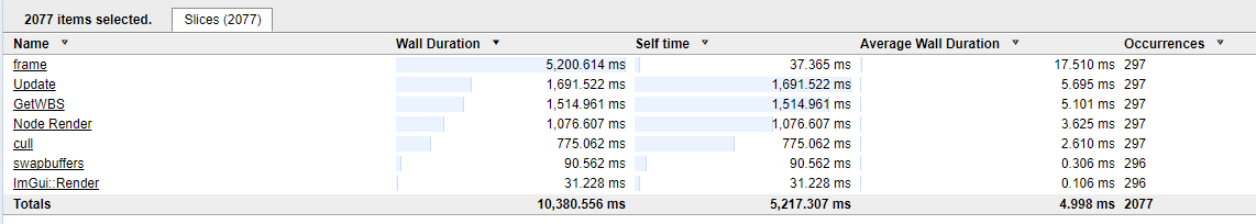
After the changes, we first verify that the code is correctly compiled and executed. Here are the previous results from the test profile:

But what happened after changing the layout in memory: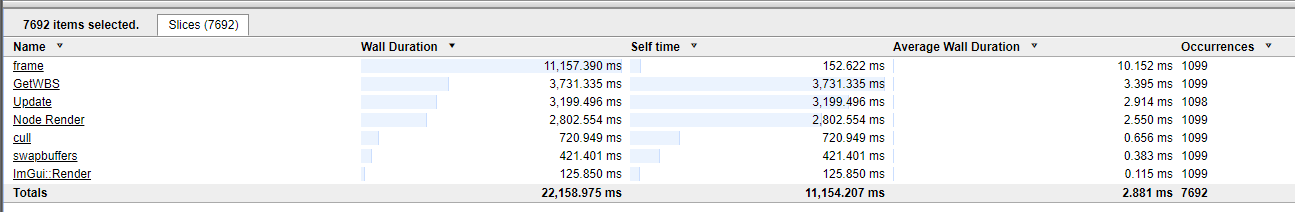

That is, we accelerated the program from 17.5 ms per frame to 10.15 ms! It has become almost twice as fast after changing only the layout of the data in memory .

Remember in this series of articles the main thing: the layout of the data in memory is critical to the performance of your program. People talk about the dangers of hasty optimizations, but, as my experience suggests, a little forethought about the relationship of data with the order of treatment and processing can greatly increase productivity. If you cannot plan the layout in advance, then try to write code conducive to the reorganization of the layout and use scheme, this will facilitate optimization. In most cases, it is not the code that hinders access to the data.

Next bottleneck

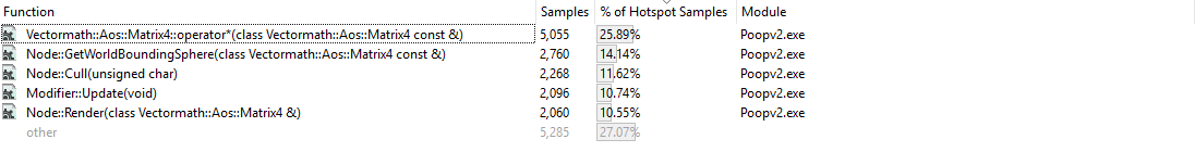
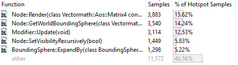
The code got faster, but is it enough? Of course not. Performance characteristics have changed, so you need to repurpose and find the next candidate for optimization. Let's compare the runs of the sampling profiler. It was:

It became:

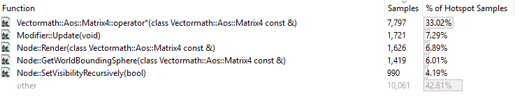
Please note that the sampling profile does not tell us if the program is now faster. It shows only the relative amount of time spent on each function. Now the matrix operator multiply function is the longest running. This does not mean that it has slowed down, just compared to others, it took longer to complete its implementation. Let's look at our sampling to see where the bottlenecks are now.

First, take a look at Modifier::Update() . The matrix is ​​no longer copied to the stack. This is advisable because we are passing the pointer to the matrix, rather than copying all of its 64 bytes.

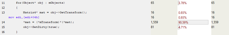
Most of the time the function works is spent on setting up the matrix multiplication call, and then on copying the result into the location of obj->mTransform (the abbreviated assembler is shown below).

The question arises: how to reduce the cost of calling a function? The answer is simple: you need to inline it. But if you look at the matrix multiplication function, it will become clear that it is ready for inline. Then what is it?

If the function is small enough, then compilers often decide to inline it automatically. But programmers can control this behavior. You can change the maximum size of the inline function, and some compilers also allow you to inline "forcibly", although this comes at a price. The size of the code may increase, and the cache will begin to slip when executing more bytes from different places.

Have a SIMD?

The matrix multiplication operator uses single floating point numbers rather than SIMD (Single Instruction Multiple Data: modern processors provide instructions that can execute one instruction in multiple data instances — like the simultaneous multiplication of four floating point numbers). Even if you tell the computer that you want to use SIMD, it will ignore you and generate similar code:

There are no SIMD instructions here, because they need data aligned by 16 bytes, and we only have 4-byte alignment. Of course, you can download the unaligned data, and then transfer it to the SIMD registers. But if the volume of SIMD processing is not too large, then the operation speed may be lower than when using a single floating point number at a time. Fortunately, we wrote a memory manager for such objects, so we can forcefully do 16-byte (or even larger) alignment for our matrices. In this example, I stopped at 16. I also forced the Vectormath library to generate only SIMD instructions.

The next time the profiler was run, it turned out that the average frame duration decreased from 10.15 to about 7 ms!

Let's look at the sampling profile:

The matrix multiplication operator has disappeared. Converting SIMD instructions reduced the size of the function so much (from 1060 bytes to about 350) that the compiler could inline it. The matrix multiplication code was included in each function that called it; now they do not invoke an instance of the multiplication function. As a side effect, the size of the code has increased (the .exe file instead of 255 began to occupy 256 KB, so I don’t care too much), but now I don’t need to copy the function parameters to the stack for their use by the called function.

Let us consider Modifier::Update() more detail:

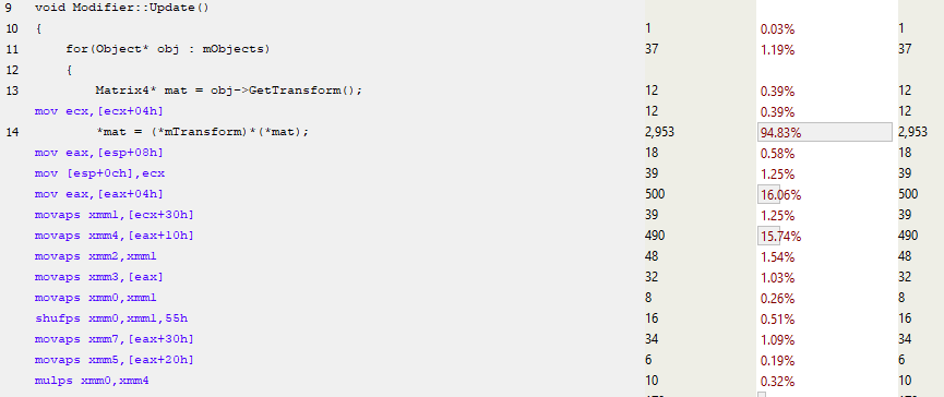
In the 13th line, the pointer to the mTransform is taken, and almost immediately after this, the matrix SIMD code uses the MOVAPS instruction (Move Aligned Single-Precision Floating-Point Values) to fill the xmm registers. So, we not only process four floating point numbers at the same time using instructions like MULPS (Multiply Packed Single-Precision Floating-Point Values), but we also load these numbers at the same time. As a result, the number of instructions in the function is greatly reduced and productivity increases. The brakes are still there, they can be attributed to cache misses, but now the performance has improved, and largely due to the improved use of instructions and inlineing. In the past, matrix multiplication was often called in the code, and now we have got rid of a significant amount of function calls.

So, we have reduced the processing time of the frame from 17.5 to about 7 ms, that is, we increased the performance by 2.5 times without degrading the code. It began to run faster without a significant increase in complexity. We have limited the way in which data is stored in memory, but we can still make low-level changes without changing the high-level code.

Additional task: virtual functions

In my presentation of 2009, I went much further than here: I broke the code, removed all the virtuals and made the code less flexible, but doubled the performance even more. I will not do it now. I'm sure we can optimize our example even more, but we will have to pay for it with readability, extensibility, portability, and maintainability. Instead, we will go through the implementation and consider the impact of virtual functions.

Virtual are functions in the base class that can be overridden in derived classes. For example, in the Object class there is a virtual function Render() , from which you can inherit and create Cube() and Elephant() objects that define the functionality of Render() . These new objects can be added to one of the Nodes, and when Render() called via the pointer in our original Object, the overridden Render() functions will be called - and they will draw a cube or an elephant on the screen.

The simplest test for our example is the SetVisibilityRecursively() method in Objects and Nodes. It is used in culling phase, when the node is entirely inside or outside the truncated figure (frustum), so that its children can simply be made visible or invisible. In the case of Object, the internal flag is just set:

 virtual void SetVisibilityRecursively(bool visibility) { m_IsVisible = visibility; } 

In the case of Node, SetVisibilityRecursively() is called for all children:

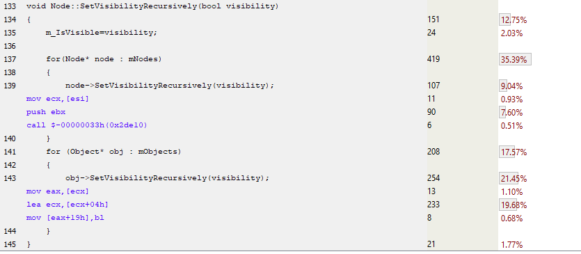
 void Node::SetVisibilityRecursively(bool visibility) { m_IsVisible = visibility; for(Object* obj : mObjects) { mObjects[i]->SetVisibilityRecursively(visibility); } } 

Here is what we see in the Node-version when analyzing the sampling profile:

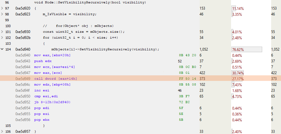
ESI is the counter for the loop, and EAX is the pointer to the next object. An interesting highlighted line is CALL DWORD [EAX + 14h]: here the virtual function is called, located in 0x14 (decimal 20) bytes from the beginning of the virtual table. Since the pointer occupies 4 bytes, and all reasonable people start counting from 0, this is a call to the fifth virtual function in the virtual table of the object. Or, as we see below, SetVisibilityRecursively() :

To call a virtual function, you need to do a little more work. A virtual table must be loaded, then a virtual function is searched in it, called, some parameters are passed to it, as well as “this” pointer.

Virtually missing virtuals

In the following code example, I have replaced virtual functions with normal ones in Nodes and Objects. This means that I need to keep two arrays in each Node (Nodes and Objects), since they are different from each other. Example:

As you can see, there are no downloads of virtual tables and dereferencing of virtual functions. In the first case, there is only a simple function call to implement Node::SetVisibilityRecursively() , and in the second case, in the implementation of Object, the function is completely inline. The compiler cannot inline virtual functions, because during compilation they cannot be determined, only at runtime. So this non-virtual implementation should work faster. Let's profile and find out.

This optimization has changed very little performance: from 6.961 to 6.963 ms. Does this mean that our code has slowed down by 0.002 ms? Not at all. This difference can be attributed to the noise background of the system, which is a personal computer running the OS, which simultaneously performs many tasks (updates my Twitter feed, checks mail, updates animation gifs on the page I forgot to close). To understand how your operating system affects the executable code, you can use the invaluable tool Windows Performance Analyzer . This software will not only show the performance of your code, but will also holistically display your entire system. So if the code unexpectedly began to be processed twice as long, then check to see if someone else is guilty of this, stealing your processor cycles. You can also read Bruce Dawson's excellent blog .

So, deleting virtual functions has very little effect on code performance. Despite the decrease in the number of searches on the virtual table and the execution of fewer instructions, the program works at the same speed. Most likely, the Miracles of Modern Equipment matter - branch prediction and speculative execution are good not only for hacking, but also to take your duplicate code and figure out how to execute it as quickly as possible.

To quote Henry Petroski (Henry Petroski):

"The most surprising achievement of the modern software industry is the continuation of the rejection of the steady and stunning success of the hardware industry."

I showed you that virtual functions are not free to use, but in this case the cost is negligible.

Summary

We profiled the sample code, identified the bottlenecks and tried to reduce their impact. After each change of the code, we redeveloped it to understand if it became worse or better (errors are useful, we learn from them). And at each stage, we better understand the code: how it is executed, how it accesses memory. Our solution minimally changes the high-level code and reduces the duration of rendering an individual frame from 17 to 7 ms. We learned that memory is slow and you need to work with hardware to write fast code.

In the third part of the series, we will look at the definition, analysis, and optimization of performance bottlenecks that we recently discovered in League of Legends .