Classification of musical compositions by performers with the help of Hidden Markov Models

Hidden Markov models (Hidden Markov Models) have long been used in speech recognition. Thanks to the chalk-cepstral coefficients (MFCC), it became possible to flip off the signal components that are not essential for recognition, significantly reducing the dimension of the features. There are many simple examples on the Internet using HMM with MFCC to recognize simple words.



After becoming acquainted with these possibilities, there appeared a desire to try out this recognition algorithm in music. Thus was born the idea of ​​the task of classifying musical compositions by performers. About attempts, some magic and the results will be discussed in this post.

Motivation

The desire to get acquainted in practice with the hidden Markov models originated a long time ago, and last year I was able to link their practical use with the course project in the magistracy.

')

During the pre-project googling, an interesting article was found telling about using HMM to classify the folk music of Ireland, Germany and France. Using a large archive of songs (thousands of songs), the authors of the article try to reveal the existence of a statistical difference between the compositions of different nations.



While studying libraries with HMM I came across the code from the Python ML Cookbook book, where, using the example of recognizing several simple words, the hmmlearn library was used, which was decided to be tested.

Formulation of the problem

In the presence of songs of several musical performers. The task is to train the classifier based on the HMM to correctly recognize the authors of the songs entering it.



Songs are presented in the format ".wav". The number of songs for different groups is different. The quality, duration of the compositions also vary.

Theory

To understand the operation of the algorithm (which parameters in which training are involved), it is necessary to at least superficially get acquainted with the theory of chalk-cepstral coefficients and hidden Markov models. More detailed information is available in the MFCC and HMM articles.



MFCC is a representation of a signal, roughly speaking, in the form of a special spectrum, from which components insignificant for human hearing are removed with the help of various filterings and transformations. The spectrum is short-lived, that is, the signal is initially divided into intersecting segments of 20-40 ms. It is assumed that on such segments of the signal frequency does not change too much. And already on these segments and magic coefficients are considered.



There is a signal







25 ms segments are taken from it.







And for each of them are calculated chalk-cepstral coefficients







The advantage of this view is that for speech recognition, it is enough to take about 16 coefficients for each frame instead of hundreds or thousands, in the case of the usual Fourier transform. Experimentally, it has been found that in order to highlight these coefficients in songs it is better to take 30-40 components each.



For a general understanding of the work of hidden Markov models, you can see the description on the wiki .



Their meaning is that there is an unknown set of hidden states$$ $ inline $ x_1, x_2, x_3 $ inline $ whose manifestation is in some sequence determined by probabilities$$ $ inline $ a_1, a_2, a_3 $ inline $ with some probabilities$$ $ inline $ b_1, b_2, b_3 $ inline $ leads to a set of observed results$$ $ inline $ y_1, y_2, y_3 $ inline $ .







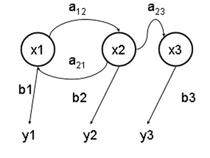
In our case, the observed results are mfcc for each frame.

The Baum-Welch algorithm (a special case of the more well-known EM algorithm) is used to find the unknown parameters of the HMM. It is he who is engaged in training the model.

Implementation

Let's start, finally, to the code. The full version is available here .



The librosa library was chosen for the calculation of the MFCC. You can also use the python_speech_features library, which, unlike librosa, implements only the functions necessary for calculating the chalk-core coefficients.



We will take the songs in the format ".wav". Below is the function for calculating the MFCC, which accepts the name of the ".wav" file as input.

def getFeaturesFromWAV(self, filename): audio, sampling_freq = librosa.load( filename, sr=None, res_type=self._res_type) features = librosa.feature.mfcc( audio, sampling_freq, n_mfcc=self._nmfcc, n_fft=self._nfft, hop_length=self._hop_length) if self._scale: features = sklearn.preprocessing.scale(features) return features.T 

On the first line, the usual download of the ".wav" file occurs. The stereo file is converted to a single channel format. librosa allows for different resampling, I stopped at res_type='scipy' .



I considered it necessary to specify three basic parameters for the calculation of attributes: n_mfcc - the number of chalk-cepstral coefficients, n_fft - the number of points for the fast Fourier transform, hop_length - the number of samples for frames (for example, 512 samples for 22kG and will give about 23ms).



Scaling is an optional step, but with it I managed to make the classifier more stable.



Let us turn to the classifier. hmmlearn turned out to be an unstable library, in which with each update something breaks. However, its compatibility with scikit is good news. At the moment (0.2.1), Hidden Markov Models with Gaussian emissions is the most working model.



Separately, I want to note the following model parameters.

 self._hmm = hmm.GaussianHMM(n_components=hmmParams.n_components, covariance_type=hmmParams.cov_type, n_iter=hmmParams.n_iter, tol=hmmParams.tol) 

Parameter n_components - determines the number of hidden states. Relatively good models can be built using 6-8 hidden states. They learn quite quickly: 10 songs take about 7 minutes on my Core i5-7300HQ 2.50GHz. But for more interesting models, I preferred to use about 20 hidden states. I tried more, but on my tests the results did not change much, and the training time increased to several days with the same number of songs.



The remaining parameters are responsible for the convergence of the EM algorithm, limiting the number of iterations, accuracy, and determining the type of covariance parameters of states.



hmmlearn is used for teaching without a teacher. Therefore, the learning process is as follows. Each class has its own model. Next, the test signal is run through each model, where it calculates the logarithmic probability of the score each model. The class that corresponds to the model that produced the highest probability, and is the owner of this test signal.



Training in the code of one model looks like this:

  featureMatrix = np.array([]) for filename in [x for x in os.listdir(subfolder) if x.endswith('.wav')]: filepath = os.path.join(subfolder, filename) features = self.getFeaturesFromWAV(filepath) featureMatrix = np.append(featureMatrix, features, axis=0) if len( featureMatrix) != 0 else features hmm_trainer = HMMTrainer(hmmParams=self._hmmParams) hmm_trainer.train(featureMatrix) 

The code runs through the subfolder folder and finds all the ".wav" files, and for each of them it considers the MFCC, which later it simply adds to the matrix of attributes. In the matrix of attributes, the row corresponds to the frame, the column corresponds to the coefficient number from the MFCC.



After the matrix is ​​filled, a hidden Markov model is created for this class, and the signs are transferred to the EM algorithm for training.



The classification looks like this.

  features = self.getFeaturesFromWAV(filepath) #label is the name of class corresponding to model scores = {} for hmm_model, label in self._models: score = hmm_model.get_score(features) scores[label] = score similarity = sorted(scores.items(), key=lambda t: t[1], reverse=True) 

We wander through all the models and count logarithmic probabilities. We get a set of classes sorted by probability. The first element and show who the most likely performer of this song.

Results and Improvements

In the training sample were selected songs of seven performers: Anathema, Hollywood Undead, Metallica, Motorhead, Nirvana, Pink Floyd, The XX. The number of songs for each of them, as well as the songs themselves, were chosen from considerations of which tests I would like to conduct.



For example, the Anathema style of the band changed greatly during their career, starting with heavy doom metal and ending with calm progressive rock. It was decided to send the songs from the first album to the test sample, and more to the training - softer songs.





Tests produced a relatively good result (4 out of 16 tests, 4 errors). Problems appeared while trying to recognize the artist by the cut part of the song.



Suddenly it turned out that when the composition itself is classified correctly, a part of it can produce a diametrically opposite result. Moreover, if this piece of composition contains the beginning of the song, then the model gives the correct result. But if it still begins with another part of the composition, then the model is entirely sure that this song does not relate to the right performer.





The solution was sought for a long time. Attempts were made to train for 50 or more hidden states (almost three days of training), the number of MFCCs increased to hundreds. But none of this solved the problem.



The problem was solved very severe, but at some level of the subconscious mind a clear idea. It consisted in randomly mixing (shuffle) rows in the matrix of features before learning. The result justified itself by slightly increasing the learning time, but producing a more robust algorithm.

  featureMatrix = np.array([]) for filename in [x for x in os.listdir(subfolder) if x.endswith('.wav')]: filepath = os.path.join(subfolder, filename) features = self.getFeaturesFromWAV(filepath) featureMatrix = np.append(featureMatrix, features, axis=0) if len( featureMatrix) != 0 else features hmm_trainer = HMMTrainer(hmmParams=self._hmmParams) np.random.shuffle(featureMatrix) #shuffle it hmm_trainer.train(featureMatrix) 

Below are the results of the model test with parameters: 20 hidden states, 40 MFCC, with component scaling and shuffle.





Result: 2 mistakes of 16 songs. In general, not bad, although mistakes scare (Pink Floyd is clearly not so heavy).



Tests with clippings of songs pass confidently.

Conclusion

The constructed classifier based on hidden Markov models shows satisfactory results, correctly identifying the performers for the majority of compositions.



All code is available here . To whom it is interesting, he can try to train models on his own compositions. According to the results, you can also try to identify the common in the music of different groups.



For a quick test on the trained compositions, you can look at the site spinning on Heroku (accepts small ".wav" files as input). The list of compositions on which the model from the site was trained is presented above in the paragraph above under the spoiler.