Mathematical model of a nuclear reactor fuel element

Introduction

A fuel element (TVEL) is the main structural element of the core of a heterogeneous nuclear reactor containing nuclear fuel [1].

In fuel rods, fission of heavy nuclei of uranium 235 or plutonium 239 occurs, accompanied by the release of thermal energy, which is then transferred to the coolant.
')
TVEL should provide heat removal from the fuel to the coolant and prevent the spread of radioactive products from the fuel to the coolant.

Therefore, the calculation of temperature fields in TVELs is an important task of designing a nuclear reactor.

This publication presents a method for calculating the temperature distribution for a core axisymmetric fuel rod made up of uranium oxide tablets.

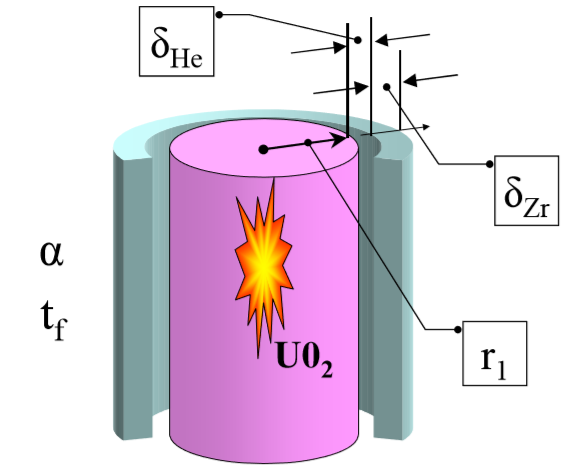
The design of axisymmetric TVELA (schematically)

Nuclear fuel is enclosed in a protective sheath of zirconium alloy - a material that weakly absorbs thermal neutrons.

Between the fuel rod and the shell there is a gap - a thin gas interlayer filled with chemically neutral and highly heat-conducting helium [2].



The power of internal sources of heat in fuel elements reaches , and thermal stress of the cooled surface, i.e. heat flux density on the surface of the shell -

It is necessary to provide effective cooling so that the temperature level is acceptable for the available materials.

In the most common civil reactors of the VVER type, cooling is carried out with water at a pressure of 15 MPa.

The saturation temperature at this pressure is 342ºC, and the temperature of the coolant (water) is about 300ºC, i.e. The fuel rods are cooled non-boiling, underheated to saturation water. The heat transfer coefficient is approximately 30,000 W / (m 2 ºC).

For uranium oxide, which is a type of ceramic nuclear fuel, the temperature can be very high, since the melting point of UO2 is 2800ºC.

However, the permissible temperature of zirconium shells is much lower - about 400º. If this limit is exceeded, destructive corrosion quickly develops in contact with water.

When designing a fuel element, it is necessary to check whether the temperatures of nuclear fuel and the containment shell do not exceed acceptable values.

The calculation is carried out at a given power of internal sources qv and given cooling conditions: water temperature tf and heat transfer coefficient α.

The design of the fuel element can be divided into two areas:

• cylindrical rod with internal sources
• gap and shell without internal sources.

Fuel rod model - cylinder with internal heat sources

Heat balance for a cylindrical fuel rod write in the form:



The right-hand side of this expression is the internal heat release in a solid cylinder with the current radius r, 0 ≤ r ≤ r1. The left side is the heat flux through the F® surface.

After substitution in the above expression ratio get the equation:

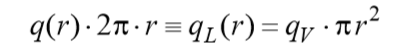. (one)

According to (1), the linear density of the heat flux increases along the radius of the fuel element due to the action of internal sources of heat.

Given the expression for the heat flux density, from the conservation equation (1) we obtain the following differential equation for the temperature field:

(2)

Variables in this equation are separated. We will integrate on the full interval:



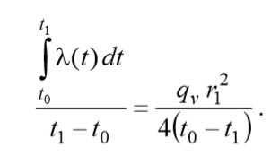
Introducing the value of the average integral thermal conductivity coefficient, we can write the calculated ratio for the temperature difference inside the fuel element in the following compact form:

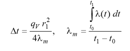(3)

Thermal conductivity of UO2 [3]:

(four)




Note that formula (3) gives the exact solution of differential equation (2) in quadratures. Numerical errors may occur in the approximate calculation of the integral.

If we take λ = const, then from (3) follows the quadratic law of temperature variation along the radius. To see this, fix the value t0 in Δt t t 0 - t1 and consider t1 as a function of radius r1.

In fact, the thermal conductivity of uranium oxide strongly depends on temperature (4) and this dependence must be taken into account in practical calculations.

We set the heat generation power qv and the surface temperature of the fuel rod t1. It is required to find the temperature in the center t0 (this is the maximum value of the temperature in the fuel element).

For such calculations, it was necessary to develop a program in Python:

 # -*- coding: utf8 -*- import numpy as np from scipy.optimize import * from scipy.integrate import quad import matplotlib.pyplot as plt def Luo2(t):#       return 8.706+(-9.11*(10**-3))*t+(3.992*(10**-6))*(t**2)+(-5.004*(10**-10))*(t**3) x= np.arange(0.0,2500.0,100.0) qv=10**9#   r1=0.0038#    def LLuo2(t1,t2):#         if abs(t1-t2)<0.001: z=Luo2(t1) else: z=(1/(t2-t1))*(quad(lambda t: Luo2(t), t1,t2)[0]) return z t1=942.413#       t0=round(fsolve(lambda t0:t0-t1-(qv*r1**2)/(4*LLuo2(t1,t0)) ,t1)[0],1) print('  t0     - %s ° '%t0) 

We get:

Temperature t0 in the center of the fuel rod -2359.2 °

So, to use the exact solution (3) of the problem of developing a mathematical model of a fuel element, it took special use of the Python –fsolve and quad modules, as well as “nested” functions.

Note that this is the easiest way to solve if it is necessary to correctly take into account the influence of the temperature dependence of the thermal conductivity of nuclear fuel.

Calculation of heat transfer through a gap filled with helium and a zirconium protective sheath

The heat released in the active rod is then transferred through the gas gap and the zirconium sheath to the cooling water.

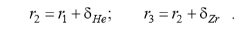
Since there are no internal heat sources in this region, the linear flow qL is kept constant, and from (1) it follows:



The thermal conductivity of helium in the gas interlayer substantially depends on the temperature:

(five)




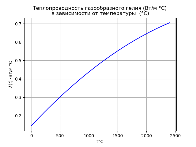
We take into account that the thermal conductivity of helium in a gas interlayer substantially depends on temperature, while at the same time the thermal conductivity of a zirconium alloy can be considered constant:



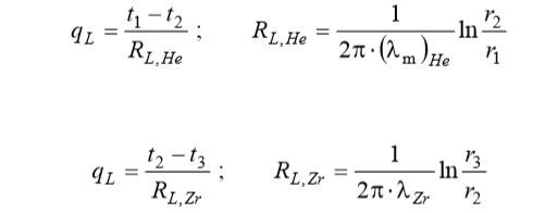
Where:



Heat transfer on the surface of the shell will be described by the Newton Richman equation: converted to linear heat flux density:

,

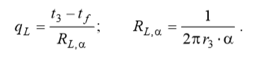where: RL, α is called linear heat transfer resistance.

The linear thermal resistances of the helium gap, the shell, and the heat transfer on the outer surface form a series of resistances through which the same (linear) heat flow qL passes:

(6)



Calculations will be elementary if the resistances are temperature independent. However, in many heat transfer tasks this is not the case.

Now we are dealing with the simplest example of nonlinear resistance, due to the strong temperature dependence of the thermal conductivity of helium in the gap.

More complex are problems with temperature-dependent heat transfer resistances (as in boiling or condensation, with free convection or radiative heat transfer).

Since the problem is quite general, we will show how to organize heat transfer calculations in such cases:

• The temperature dependencies of the materials should be specified as functions that other program blocks can access.
• thermal resistance should be recorded taking into account the temperature dependence
• should be formed for a series circuit of a system of equations, such as (6), containing unknown temperatures t1, t2, t3.

For such complex calculations, it was necessary to develop a Python program containing a chain of nested functions:

 # -*- coding: utf8 -*- import numpy as np from scipy.optimize import * from scipy.integrate import quad import matplotlib.pyplot as plt def Luo2(t):#       return 8.706+(-9.11*(10**-3))*t+(3.992*(10**-6))*(t**2)+(-5.004*(10**-10))*(t**3) x= np.arange(0.0,2500.0,100.0) qv=10**9#   r1=0.0038#    def LLuo2(t1,t2):#         if abs(t1-t2)<0.001: z=Luo2(t1) else: z=(1/(t2-t1))*(quad(lambda t: Luo2(t), t1,t2)[0]) return z t1=942.413#       t0=round(fsolve(lambda t0:t0-t1-(qv*r1**2)/(4*LLuo2(t1,t0)) ,t1)[0],1) print('  t0      ° -%s'%t0) def Lhe(t):#      return 0.146+3.339*(10**-4)*t-4.219*(10**-8)*t**2 def LLhe(t1,t2):#        if abs(t1-t2)<0.001: z=Lhe(t1) else: z=(1/(t2-t1))*(quad(lambda t: Lhe(t), t1,t2)[0]) return z dzr=0.00065#      dhe=0.0001#  ,   r2=r1+dhe#      r3=r2+dzr#      Lzr=20#   tf=300#    alf=30000#  RL_alf=1/(alf*2*np.pi*r3)#    RL_Zr=(1/(2*np.pi*Lzr)*np.log(r3/r2))#    def RL_He(t1,t2):#   return (1/(2*np.pi*LLhe(t1,t2))*np.log(r2/r1)) ql=qv*np.pi*r1**2#         def fun(t1,t2,t3): #          z=(t1-tf-ql*(RL_He(t1,t2)+RL_Zr+RL_alf)) return z t3=tf+ql*RL_alf t2=t3+ql*RL_Zr tt0=400#    t1 t1=fsolve(lambda t1:fun(t1,t2,t3),tt0)[0]#  t1 print(' t1      ::%s °'%round(t1,1)) print(' t2      : %s °'%round(t2,1)) print(' t3      : %s °'%round(t3,1)) 

We get:

Temperature t0 in the center of the fuel rod: 2359.2 °
The temperature t1 of the surface of the fuel rod of uranium oxide: 942.4 ° C
Temperature t2 of the inner surface of the zirconium shell: 408.5 °
Temperature t3 of the outer surface of the zirconium shell: 352.9 °

Temperature distribution in the fuel rod

 # -*- coding: utf8 -*- import numpy as np from scipy.optimize import * from scipy.integrate import quad import matplotlib.pyplot as plt def Luo2(t):#       return 8.706+(-9.11*(10**-3))*t+(3.992*(10**-6))*(t**2)+(-5.004*(10**-10))*(t**3) x= np.arange(0.0,2500.0,100.0) qv=10**9#   r1=0.0038#    def LLuo2(t1,t2):#         if abs(t1-t2)<0.001: z=Luo2(t1) else: z=(1/(t2-t1))*(quad(lambda t: Luo2(t), t1,t2)[0]) return z t1=942.413#       t0=round(fsolve(lambda t0:t0-t1-(qv*r1**2)/(4*LLuo2(t1,t0)) ,t1)[0],1) print('  t0     : %s °'%t0) def Lhe(t):#      return 0.146+3.339*(10**-4)*t-4.219*(10**-8)*t**2 def LLhe(t1,t2):#        if abs(t1-t2)<0.001: z=Lhe(t1) else: z=(1/(t2-t1))*(quad(lambda t: Lhe(t), t1,t2)[0]) return z dzr=0.00065#      dhe=0.0001#  ,   r2=r1+dhe#      r3=r2+dzr#      Lzr=20#    tf=300#    alf=30000#  RL_alf=1/(alf*2*np.pi*r3)#    RL_Zr=(1/(2*np.pi*Lzr)*np.log(r3/r2))#    def RL_He(t1,t2):#   return (1/(2*np.pi*LLhe(t1,t2))*np.log(r2/r1)) ql=qv*np.pi*r1**2#         def fun(t1,t2,t3): #          z=(t1-tf-ql*(RL_He(t1,t2)+RL_Zr+RL_alf)) return z t3=tf+ql*RL_alf t2=t3+ql*RL_Zr tt0=400#    t1 t1=fsolve(lambda t1:fun(t1,t2,t3),tt0)[0]#  t1 print(' t1      : %s °'%round(t1,1)) print(' t2     : %s °'%round(t2,1)) print(' t3     : %s °'%round(t3,1)) def eq(t,r):#           return t0-t-qv*r**2/(4*LLuo2(t,t0)) def t_tuel(r):#         return fsolve(lambda t:eq(t,r) ,t0)[0] def t_out(r):#            if r2<r<=r3: z=t2+(t3-t2)*np.log(r/r2)/np.log(r3/r2) elif r1<=r<=r2: z=t1+(t2-t1)*np.log(r/r1)/np.log(r2/r1) elif r>r3: z=tf return z tt1=[t_tuel(r) for r in np.arange(0.0,r1+0.0001,0.0001)] rr1=np.arange(0.0,r1+0.0001,0.0001) tt2=[t_out(r) for r in np.arange(r1,r3+0.001,0.0001)] rr2=np.arange(r1,r3+0.001,0.0001) plt.title('     ') plt.plot(rr1,tt1, color='r',linewidth=2, label=' 0<=r<=r1') plt.plot(rr2,tt2, color='b',linewidth=2, label='r1<r<=r3+0.001 ') plt.plot(0,t0,'o',label='t0=%s° '%t0) plt.plot(r1, t_tuel(r1),'o',label='t1=%s °'%round(t_tuel(r1),1)) plt.plot(r2, t_out(r2),'o',label='t2=%s °'%round(t_out(r2),1)) plt.plot(r3, t_out(r3),'o',label='t3=%s °'%round(t_out(r3),1)) plt.plot(r3+0.001, t_out(r3+0.001),'o',label='tf=%s °'%round(t_out(r3+0.001),1)) plt.xlabel("r  .") plt.ylabel("t  °") plt.grid(True) plt.legend(loc='best') plt.show() 

We get:



The results of the calculation of the fuel element are presented in the graph as the temperature distribution over the radius. The focus of the evaluation of the results should be given to two values:

1. maximum temperature of nuclear fuel t0. The maximum limit value can be estimated as the melting point of uranium oxide, approximately 2800 ° C,
2. surface temperature of the containment t3, where contact with water occurs. The permissible temperature of zirconium alloy shells is about 400º. At higher temperatures, destructive corrosion quickly develops in contact with water.

Thus, the considered temperature regime is close to the ultimate in thermal stress.

findings

A means of a freely distributed Python programming language using the quad, fsole modules and a system of nested functions was developed a mathematical model for an axisymmetric fuel element of a nuclear reactor.

Links

1. Fuel element.
2. Heat and mass transfer in power plants.
3. Properties of uranium oxide, KTP of nitrous oxide.