Profiling: measurement and analysis

Hi, I'm Tony Albrecht, an engineer at Riot. I like to profile and optimize. In this article I will talk about the basics of profiling, as well as analyze the example of C ++ code during its profiling on a Windows machine. We will start with the simplest and will gradually delve into the intrinsic of the CPU. When we meet the possibilities to optimize, we will implement the changes, and in the next article we will analyze real examples from the code base of the game League of Legends. Go!

Code review

First, take a look at the code that we are going to profile. Our program is a simple little OpenGL renderer, an object-oriented, hierarchical scene tree. I resourcefully called the main object Object'om - everything in the scene is inherited from one of these base classes. In our code, only Node, Cube and Modifier are inherited from Object.

Cube is an Object that renders itself on the screen as a cube. Modifier is an Object that “lives” in the scene tree and, being Updated, transforms the Objects added to it. A Node is an Object that can contain other Objects.

The system is designed so that you can create a hierarchy of objects by adding cubes to the nodes, as well as one node to the other nodes. If you convert a node (using a modifier), then all objects contained in the node will be converted. With this simple system, I created a tree of cubes rotating around each other.

I agree, the proposed code is not the best implementation of the scene tree, but that's okay: this code is needed for subsequent optimization. In fact, this is a direct porting of an example for PlayStation3®, which I wrote in 2009 to analyze the performance of Pitfalls of Object Oriented Programming . In part, we can compare our today's article with a 9-year-old article and see if the lessons we learned once for PS3 apply to modern hardware platforms.

But back to our cubes. The above gif shows about 55 thousand rotating cubes. Please note that I do not profile the rendering of the scene, but only the animation and culling during the transfer to render. Libraries involved in creating an example: Dear Imgui and Vectormath from Bullet are both free. For profiling, I used AMD Code XL and a simple instrumented profiler, hastily built for this article.

Before getting down to business

Units

First I want to discuss performance measurement. Often, games per second use frames per second (FPS). This is a good indicator of performance, but it is useless when analyzing parts of a frame or comparing improvements from different optimizations. Suppose, “the game is now running at 20 frames per second faster!” - is that even how much faster?

Depends on the situation. If we had 60 FPS (or 1000/60 = 16,666 milliseconds per frame), and now it is 80 FPS (1000/80 = 12.5 ms per frame), then our improvement is 16.666 ms - 12.5 ms = 4.166 ms on frame. This is a good increase.

But if we had 20 FPS, and now it's 40 FPS, then the improvement is already (1000/20 - 1000/40) = 50 ms - 25 ms = 25 ms per frame! This is a powerful performance boost that can turn a game from “unplayable” to “acceptable.” The problem with the FPS metric is that it is relative, so we will always use milliseconds. Is always.

Measurement

There are several types of profilers, each with its own advantages and disadvantages.

Control Profilers

For instrumented profiling, the programmer must manually mark a piece of code whose performance needs to be measured. These profilers capture and save the start and end times of the profiled fragment, focusing on unique markers. For example:

void Node::Update() { FT_PROFILE_FN for(Object* obj : mObjects) { obj->Update(); } } 

In this case, FT_PROFILE_FN creates an object that records the time of its creation, and then the destruction when it FT_PROFILE_FN out of scope. These times along with the name of the function are stored in an array for further analysis and visualization. If you try, you can implement the visualization in the code or - a little easier - in a tool like Chrome tracing .

Measurement profiling is great for visually displaying the performance of a code and detecting its bursts. If the performance characteristics of the application are presented in the form of a hierarchy, then you can immediately see which functions work most slowly the most, which ones cause the most other functions, which ones have the most duration of execution, etc.

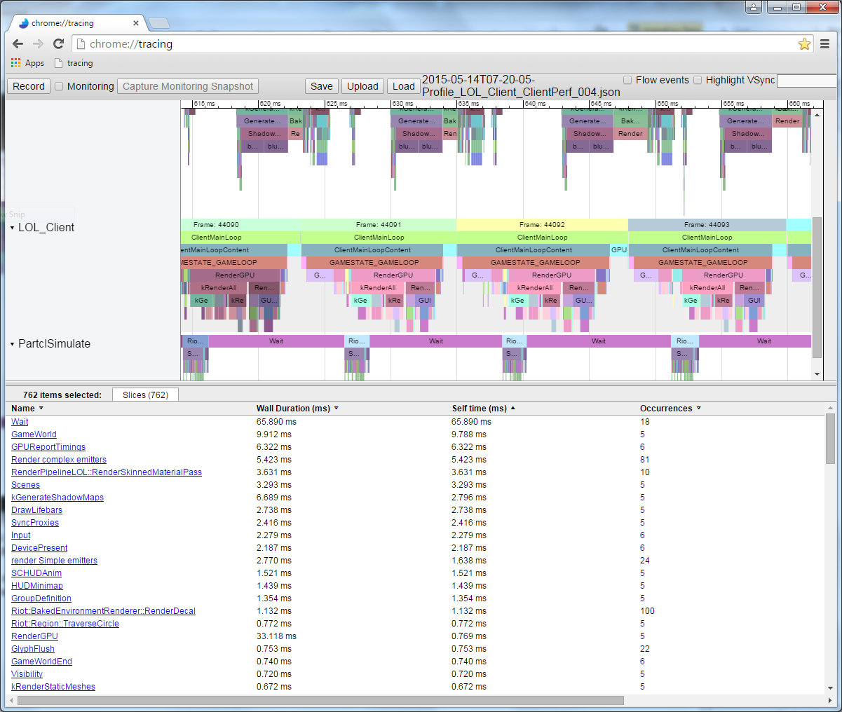
In this illustration, each colored plate corresponds to a function. Dies located directly under the other dies denote functions that are called "upstream" functions. The length of the plate is proportional to the duration of the execution of the function.

Although instrumentation profiling provides valuable visual information, it still has flaws. It slows down the execution of the program: the more you measure, the slower the program becomes. Therefore, when writing a measurement profiler, try to minimize its impact on application performance. If you skip the slow function, a large gap in the profile will appear. Also, you will not get information about the speed of each line of code: you can easily mark only visibility areas, but the overhead of measuring and profiling usually nullifies the contribution of individual lines, so measuring them is simply useless.

Sampling Profilers

Sampling profiles request the execution status of the process you want to profile. They periodically save the program counter (PC), showing which instruction is currently being executed, and also keep the stack, so you can find out what functions the function called that contains the current instruction called. All this information is useful, since the function or lines with the largest number of samples will be the slowest function or lines. The longer the sampling profiler is running, the more samples of instructions and stacks are collected, which improves the results.

Sampling profilers allow you to collect very low-level performance characteristics of the program and do not require manual intervention, as is the case with instrumentation profilers. In addition, they automatically cover the entire execution status of your program. These profilers have two major drawbacks: they are not very useful for defining bursts for each frame, and also do not allow to know when a certain function was called relative to other functions. That is, we get less information about hierarchical calls compared to a good measuring profiler.

Specialized Profilers

These profilers provide specific process information. Usually they are associated with hardware elements like a CPU or a video card that are capable of generating specific events if something of interest is happening, such as a cache miss or an erroneous branch prediction. Equipment manufacturers are building the ability to measure these events so that it is easier for us to find out the reasons for poor performance; therefore, to understand these profiles, knowledge of the hardware used is needed.

Game Profilers

At a much more general level, profilers designed for specific games can calculate, say, the number of minions on the screen or the number of visible particles in a character's field of view. Such profilers are also very useful, they will help to identify high-level errors in the game logic.

Profiling

Profiling an application without a benchmark does not make sense, so when optimizing, you need to have a reliable test script at hand. This is not as easy as it sounds. Modern computers perform not only your application, but at the same time dozens, if not hundreds of other processes, constantly switching between them. That is, other processes may slow down the process you are profiling as a result of competition for accessing devices (for example, several processes are trying to be counted from disk) or for processor / video card resources. So in order to get a good starting point, you need to run the code through several profiling operations before you even get down to the task. If the results of the runs are very different, then you have to figure out the reasons and get rid of the variability or at least reduce it.

Having achieved the smallest possible variation in results, do not forget that small improvements (less than the available variation) will be difficult to measure, because they can be lost in the "noise" of the system. Suppose a particular scene in the game is displayed in the range of 14-18 ms per frame, an average of 16 ms. You spent two weeks optimizing some function, repurposed it and got 15.5 ms per frame. Has it become faster? To find out exactly, you will have to chase the game many times, profiling this scene and calculating the arithmetic mean and plotting the trend. In the application described here, we measure hundreds of frames and average the results to get a fairly reliable value.

In addition, many games are executed in several streams, the order of which is determined by your hardware and operating system, which can lead to non-deterministic behavior or at least to different duration of execution. Do not forget about the influence of these factors.

In connection with the above, I collected a small test script for profiling and optimization. It is simple to understand, but complex enough to have a resource of significant performance improvement. Note that for the sake of simplicity, I turned off rendering when profiling, so that we only see the computational costs associated with the central processor.

Profile the code

Below is the code that we will optimize. Remember that one example will only teach us about profiling. You will certainly encounter unexpected difficulties when profiling your own code, and I hope that this article will help you create your own diagnostic framework.

 { FT_PROFILE("Update"); mRootNode->Update(); } { FT_PROFILE("GetWBS"); BoundingSphere totalVolume = mRootNode->GetWorldBoundingSphere(Matrix4::identity()); } { FT_PROFILE("cull"); uint8_t clipFlags = 63; mRootNode->Cull(clipFlags); } { FT_PROFILE("Node Render"); mRootNode->Render(mvp); } 

I added the FT_PROFILE() control macro to different scopes to measure the duration of execution of different parts of the code. Below we will talk more about the purpose of each fragment.

When I ran the code and recorded the data from the measured profile, I received the following picture in Chrome: // tracing:

This is a single frame profile. Here we see the relative duration of each function call. Please note that you can see the order of execution. If I measured the functions that are called by these function calls, they would be displayed under the dies of the parent functions. For example, I measured Node::Update() and got the following recursive call structure:

The duration of the execution of one frame of this code when measured varies by a couple of milliseconds, so we take the arithmetic mean for at least several hundred frames and compare it with the original standard. In this case, 297 frames were measured, the average value was 17.5 ms, some frames were executed up to 19 ms, and others were slightly less than 16.5 ms, although in each of them almost the same thing was done. Such is the implicit variation in frames. Repeated run and comparison of results consistently give us about 17.5 ms, so this value can be considered as a reliable starting point.

If you disable check marks in the code and run it through the AMD CodeXL sampling profiler, you get the following picture:

If we analyze the five most "sought-after" functions, we get:

It seems that the slowest function is matrix multiplication. It sounds logical, because for all these rotations, the function has to perform a bunch of calculations. If you look closely at the stack hierarchy with a couple of illustrations above, you will notice that the matrix multiplication operator is called by Modifier::Update() , Node::Update() , GetWorldBoundingSphere() and Node::Render() . It is called so often and from so many places - so this operator can be considered a good candidate for optimization.

Matrix :: operator *

If you analyze the code responsible for multiplication using the sampling profiler, you can find out the "cost" of each line.

Unfortunately, the length of the matrix multiplication code is just one line (for the sake of efficiency), so this result does little for us. Or is it not so little?

If you look at the assembler, you can identify the prologue and epilogue of the function.

This is the cost of an internal function call instruction. In the prologue, a new stack space is set (ESP is the current stack pointer, EBP is the base pointer for the current stack frame), and the epilogue is cleared and returned. Each time you call a function that is not inline and uses any stack space (that is, it has a local variable), all these instructions can be inserted and called.

Let's expand the rest of the function and see what matrix multiplication actually does.

Wow, a lot of code! And this is only the first page. The full function takes more than a kilobyte of code with 250–300 instructions! Let's analyze the beginning of the function.

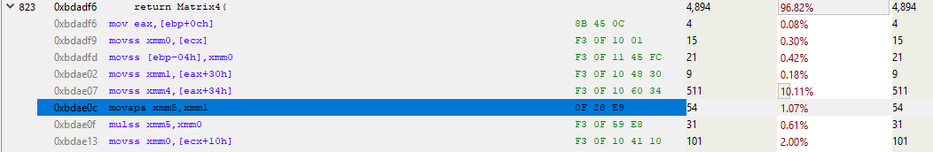
The line above the highlighted blue color takes about 10% of the total execution time. Why is it performed much slower than its neighbors? This MOVSS instruction takes from the memory at eax + 34h a floating point value and puts in the xmm4 register. The line above does the same thing with the xmm1 register, but much faster. Why?

It's all a cache miss.

We will understand in more detail. Sampling of individual instructions is applicable in a variety of situations. Modern processors at any time carry out several instructions, and within one clock cycle many instructions can be re-sorted. Even event-based sampling can attribute events to the wrong instruction. So when analyzing sampler assembly, you need to be guided by some kind of logic. In our example, the most sampled instruction may not be the slowest. We can only speak with a certain degree of confidence about the slow work of something related to this line. And since the processor performs a number of MOVs in and out of memory, suppose that these MOVs are to blame for the poor performance. To verify this, you can run a profile with enabled event-based sampling for cache misses and look at the result. But for the time being, we will trust our instincts and drive out the profile based on the cache miss hypothesis.

Passing the L3 cache takes more than 100 cycles (in some cases, several hundred cycles), and the L2 cache miss is about 40 cycles, although it all depends heavily on the processor. For example, x86- instructions take from 1 to about 100 cycles, with the majority being less than 20 cycles (some division instructions on some gland work rather slowly). On my Core i7, the instructions for multiplying, adding and even dividing took several cycles. The instructions fall into the pipeline, so that several instructions are processed simultaneously. This means that one miss of the L3 cache — loading directly from memory — can take hundreds of instructions to execute. Simply put, reading from memory is a very slow process.

Modifier :: Update ()

So, we see that accessing memory slows down the execution of our code. Let's go back and see what in the code leads to this conversion. The test profiler shows that Node::Update() is running slowly, and from the sampling profiler report about the stack, it is obvious that the Modifier::Update() function is especially slow. With this, we will start optimization.

 void Modifier::Update() { for(Object* obj : mObjects) { Matrix4 mat = obj->GetTransform(); mat = mTransform*mat; obj->SetTransform(mat); } } 

Modifier::Update() passes through the vector of pointers to Objects, takes their transform matrix, multiplies it by the mTransform Modifier matrix, and then applies this transformation to Objects. In the above code, the conversion is copied from object to stack, multiplied, and then copied back.

GetTransform() simply returns a copy of mTransform , while SetTransform() copies the new matrix to mTransform and sets the mDirty state of this object:

 void SetDirty(bool dirty) { if (dirty && (dirty != mDirty)) { if (mParent) mParent->SetDirty(dirty); } mDirty = dirty; } void SetTransform(Matrix4& transform) { mTransform = transform; SetDirty(true); } inline const Matrix4 GetTransform() const { return mTransform; } 

The inner data layer of this Object looks like this:

 protected: Matrix4 mTransform; Matrix4 mWorldTransform; BoundingSphere mBoundingSphere; BoundingSphere mWorldBoundingSphere; bool m_IsVisible = true; const char* mName; bool mDirty = true; Object* mParent; }; 

For clarity, I colored the entries in the memory of the Node object:

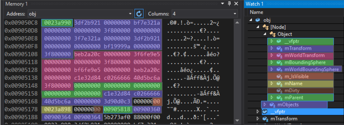
The first entry is a virtual table pointer. This is part of the implementation of inheritance in C ++: a pointer to an array of function pointers that act as virtual functions for this particular polymorphic object. For Object, Node, Modifier, and any class that inherits from the base class, there are different virtual tables.

After this 4-byte pointer, there is a 64-byte array of floating-point numbers. Behind the mTransform matrix goes the mTransform matrix, and then the two bounding spheres. Note that the next entry, m_IsVisible , is single-byte; it takes 4 full bytes. This is normal, since the next entry is a pointer that must have at least 4-byte alignment. If, after m_IsVisible put another boolean value, then it would be packed into available 3 bytes. Next comes the mName pointer (with 4-byte alignment), then the boolean mDirty (also loosely packed), then the pointer to the parent Object. All of this is Object-specific data. The subsequent mObjects vector mObjects belongs to the Node vector and occupies 12 bytes on this platform, although on other platforms it may be of a different size.

If we look at the Modifier::Update() code, we will see what could be the cause of a cache miss.

 void Modifier::Update() { for(Object* obj : mObjects) { 

To begin with, we note: the mObjects vector is an array of pointers to Objects, which are dynamically allocated in memory. Iteration over this vector works well with the cache (the red arrows in the illustration below), since the pointers follow one after the other. There are a few blunders there, but they point to something that is probably not adapted to work with the cache. And since each Object is placed in memory with a new pointer, we can only say that our interference is somewhere in memory.

When we get a pointer to an Object, we call GetTransform() :

 Matrix4 mat = obj->GetTransform(); 

This inline function simply returns a copy of mTransform Object, so the previous line is equivalent to this:

 Matrix4 mat = obj->mTransform; 

As you can see in the diagram, the Objects referenced by the pointers in the mObjects array are scattered across memory. Every time we add a new Object and call GetTransform() , this certainly results in a cache miss when loaded into mTransform and placed on the stack. On the hardware I use, the cache line is 64 bytes, so if you're lucky and the object starts 4 bytes before the 64-byte border, mTransform will be loaded into the cache all at once. But more likely is the situation when loading mTransform will result in two cache slips. From the sampling profile of Modifier::Update() it is obvious that the matrix is ​​aligned randomly.

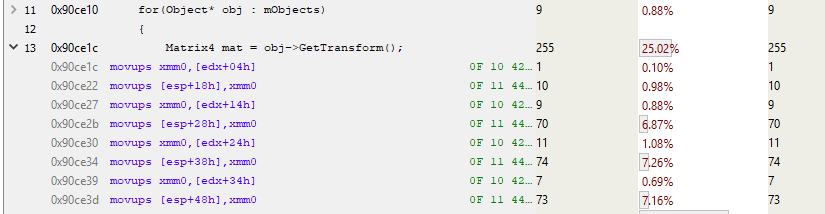
In this snippet, edx is the location of the Object. And as we know, mTransform begins 4 bytes before the beginning of the object. So this code copies mTransform to the stack (MOVUPS copies 4 floating-point values ​​to the register). Pay 7% access to three MOVUPS instructions. This suggests that cache misses are also found in the case of MOVs. I do not know why the first MOVUPS per stack does not take as much time as the others. It seems to me that the “costs” are simply transferred to subsequent MOVUPS due to the peculiarities of pipelining instructions. But in any case, we received evidence of the high cost of memory access, so we will work with it.

 void Modifier::Update() { for(Object* obj : mObjects) { Matrix4 mat = obj->GetTransform(); mat = mTransform*mat; obj->SetTransform(mat); } } 

After the matrix is ​​multiplied, we call Object::SetTransform() , which takes the result of the multiplication (freshly placed onto the stack) and copies it into the Object instance. Copying is fast, because the conversion is already cached, but SetDirty() is slow because it reads the mDirty flag, it is probably not in the cache. So for testing and, possibly, determining this one byte, the processor has to read the surrounding 63 bytes.

Conclusion

If you have read to the end - well done! I know, at first it is difficult, especially if you are not familiar with the assembler. But I highly recommend taking the time and see what the compilers do with the code they write. To do this, you can use the Compiler Explorer .

We have gathered some evidence that the main cause of performance problems in our example code is memory access pointers. Next, we minimize the cost of memory access, and then measure the performance again to see if it was possible to achieve improvement. This we will do next time.